Physical Address
304 North Cardinal St.
Dorchester Center, MA 02124
Physical Address
304 North Cardinal St.
Dorchester Center, MA 02124
Topology is a branch of mathematics devoted to studying sets, and functions defined on those sets. When dealing with the real number line, the subsets we are going to focus on are the open intervals (a, b) and the closed intervals [a, b]. Half-open intervals (a, b] and [a, b) will make appearances, as will unbounded intervals. Naturally, we will also consider unions and intersections of these intervals. The functions we will focus on are real-valued functions that are defined on those subsets previously mentioned.
As will be seen in this section, and in later chapters, what properties a function has will depend on what kind of set it is defined on. In the next few problems, we’ll see examples where inclusion or exclusion of an interval’s boundary points will have important implications.
Consider the function
y = 2x + 3.
| a.) | Does this function achieve a maximum over the following intervals? [-1, 2] [-1, 2) (-1, 2] (-1, 2) |
| b.) | Does this function achieve a minimum over the following intervals? [-1, 2] [-1, 2) (-1, 2] (-1, 2) |
| c.) | Does this function have a maximum or a minimum over all of ℝ? |
Consider the function
y = x2 – x – 6.
| a.) | Does this function achieve a maximum over the following intervals? [0, 2] [0, 2) (0, 2] (0, 2) |
| b.) | Does this function achieve a minimum over the following intervals? [0, 2] [0, 2) (0, 2] (0, 2) |
| c.) | Does this function have a maximum or a minimum over all of ℝ? |
Consider the function
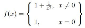
| a.) | Does this function achieve a maximum or minimum over (-∞, -1)? |
| b.) | Does this function achieve a maximum or minimum over [1, ∞)? |
| c.) | Does this function achieve a maximum or minimum over (0, 1)? |
| d.) | Does this function achieve a maximum or minimum over [0, 1]? |
Consider the function
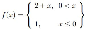
| a.) | Notice that f(0.1) = 2.1, and that f(2) = 4. Furthermore, notice that 2.1 ≤ 2.5 ≤ 4. Does this function ever achieve the value 2.5 over the interval (0, 2]? |
| b.) | Does this function take on every value in (2, 4] over the interval (0, 2]? |
| c.) | Notice that f(0) = 1, and that f(2) = 4. Furthermore, notice that 1 ≤ 1.5 ≤ 4. Does this function ever achieve the value 1.5 over the interval [0, 2]? |
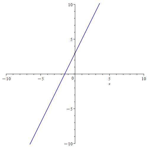
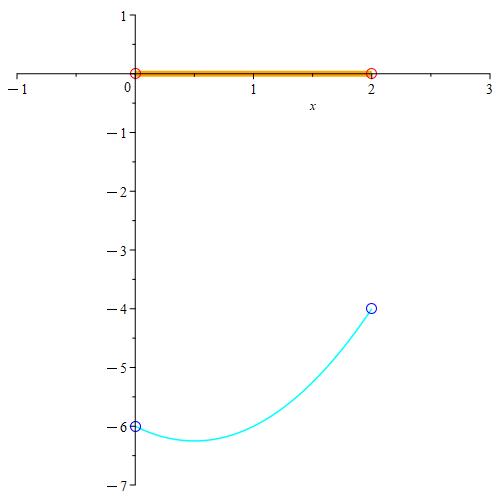
Figure 1: The function y = 2x + 3 is unbounded in either direction.
It will help to see what we’re dealing with, so let’s plot this function over the desired intervals.
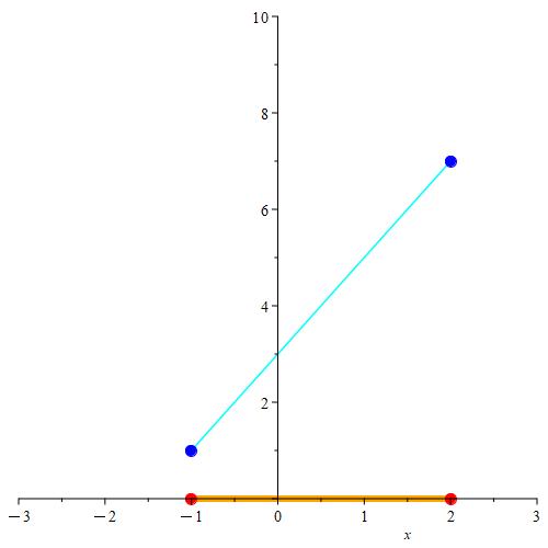
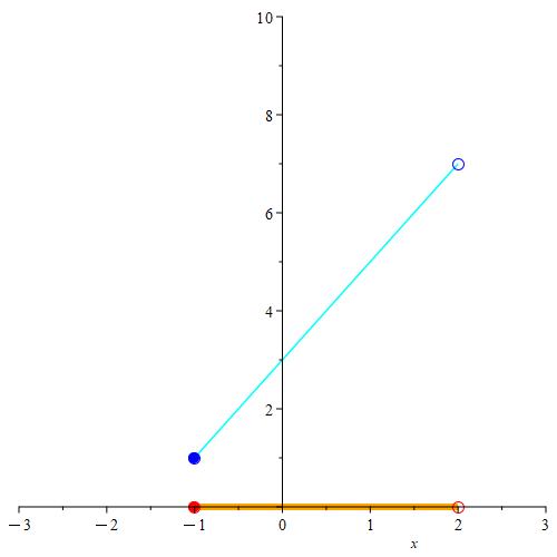
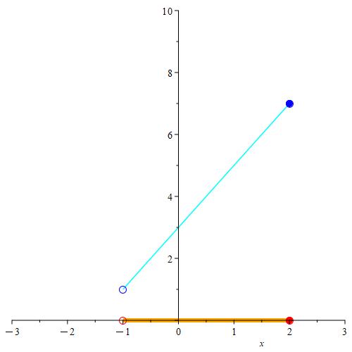
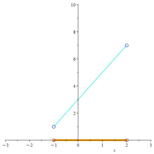
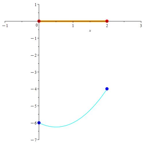
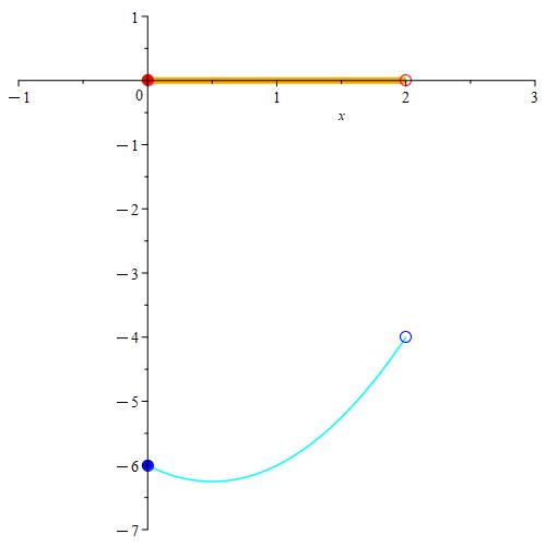
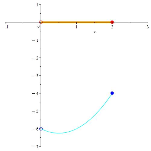
In these figures, we plotted the function in cyan, and the desired interval in orange. The function’s endpoints are in blue, while the interval’s endpoints are in red. Solid endpoints mean that the endpoint is included, while empty circles represent excluded endpoints. The captions describe the intervals over which the function was plotted, and the interval of values produced by f(x). With that taken care of, let’s answer the questions at hand.
a.)
When looking for maximums, we note that the function is strictly increasing as x increases, so we only have to consider the right endpoints. For i and iii , we see that a maximum value is achieved at x = 2, where f(2) = 7.
However, for ii and iv, 2 is not included in the interval. For any number x ∈ [-1, 2), we also have that
(x + 2)/2 ∈ [-1, 2). This is also the case for interval (-1, 2). This means that neither [-1, 2) nor (-1, 2) have maximum values. Hence, f(x) will not have a maximum. The main issue here is that the supremum is not included in the interval.
b.)
In this case, we’re looking for minimums, so we’re examining the left endpoints.
Both i and ii achieve their minimum value over the specified interval, while iii and iv do not. This time, it’s because i and ii include their infima, while iii and iv do not.
c.)
In this case the problem was because the function is unbounded. Without an upper bound or a lower bound, there can be no maximum or minimum respectively.
Let’s take a moment to reflect on what we’ve just figured out. When looking for a maximum or a minimum, we needed to look at the boundary points of the interval over which a function was defined. When we looked for maxima and minima over ℝ, we came up empty-handed because the function’s output interval did not have any supremum or infimum. We needed to make sure that the function’s input interval was bounded in order to ensure the existence of a supremum and infimum.
When the input interval was bounded, we only achieved maxima or minima when the suprema or infima were in the input interval respectively.
The next example show what happens when a function has an extreme value over the entire real line.
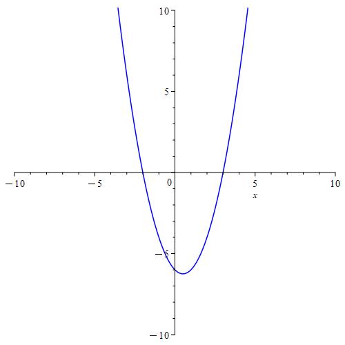
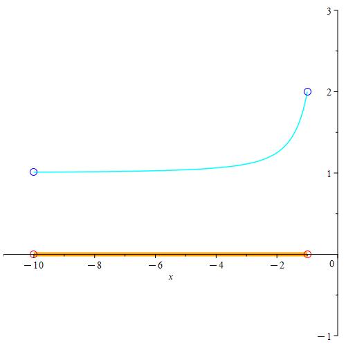
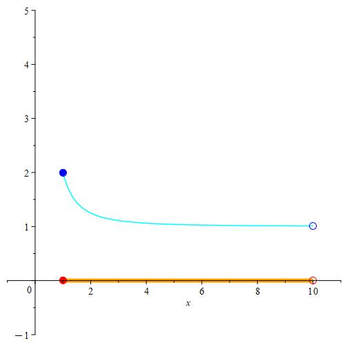
Figure 2: While f(x) from example 2 is unbounded above, there is a lower bound at y = -6.25, which occurs at x = 0.5.
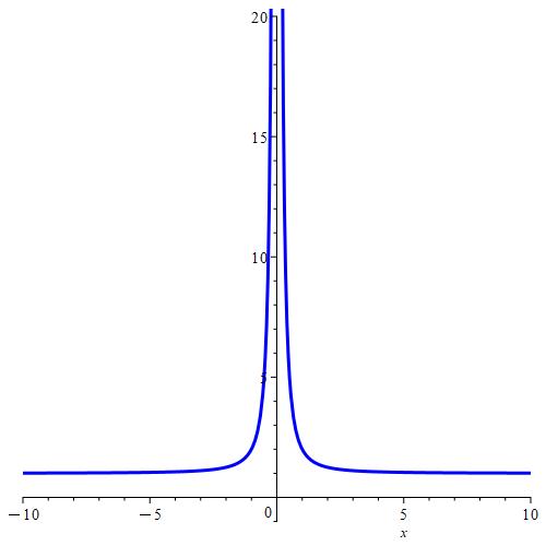
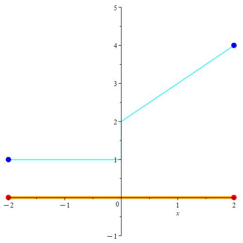
Figure 3: This function grows without bound as x gets close to 0. We get around this by making it one piece of a piece-wise defined function. We fill in the gap by simply defining f(0) = 1
This time, we’re dealing with a parabola. We’re interested only in a very narrow portion of it.
a.)
As with Solution 1, we look to see if the right endpoints are included or not. Here, i and iii include the right endpoints, so they do achieve a maximum value. ii and iv do not.
b.)
In Figure 2 above, we noted that the minimum value of this function over all of ℝ is y = -6.25, which occurs at x = 0.5. In i and ii, the left endpoints all occur at x = 0, where y = -6. The domains used for iii and iv do not include their left boundary points, but all values that are close to x = 0 in those cases are close to y = -6, which is still larger than -6.25. Since 0.5 is included in all domains, and because -6.25 < -6, this function achieves a minimum value.
c.)
As noted in Figure 2, the function is unbounded above, so no maximum is achieved. However, there is a minimum value over all of ℝ. That value is y = -6.25, which occurs at x = 0.5.
For Problem 2, we considered domains over which the function was not always increasing or decreasing. Here, the function decreases from x = 0 to x = 0.5, and increases from 0.5 to 2. As such, a minimum occurred at an x value that was “inside”, and not at a boundary of the interval.
In this case then, a minimum was achieved even when some of the domain’s boundary points were not included. However, whether a maximum value was achieved still; depended on whether or not the boundary points were included. Not surprisingly then, a function’s behavior over an interval also determines whether or not a maximum or minimum is achieved over that interval.
In Problems 1 and 2, the only interval that we could guarantee existence of a maximum or minimum was over a closed interval. Even if a global maximum or minimum does not exist within the input interval, having the boundary points included makes it so that there are endpoints, which is where a maximum or minimum would reside if no point in the domain’s “interior” resulted in a maximum or minimum.
The previous two functions did not have any breaks or gaps in their graphs. The next example will show what happens when a function’s graph has asymptotes.
Here, we’re looking at this function over several different intervals that are bordering the value x = 0. Of course, this function is “ill-behaved” at x = 0 because it grows without bound near x = 0. Let’s take a look.


a.)
Here, no maximum or minimum are achieved. The infimum of the range is 1, and the supremum is 2.
b.)
Here, the maximum value obtained in the range is 2. Since the input interval contains it’s infimum value, this is not surprising. However, since the output interval is unbounded to the right, there is no minimum value achieved.
c.)
Here, no maximum or minimum is achieved. The function increases without bound as x approaches 0 from the right, which is why there is no maximum value. There is no minimum because again, the supremum of the input interval is not included in the input interval.
d.)
This one is a little weird. There is no maximum value because the function grows without bound as x approaches 0 from the right. This time, 0 is included in the input interval, but f(0) is defined to be 1. The other boundary point at x = 1 is included, but f(1) = 2, which is greater than 1. Here, a minimum value is achieved.
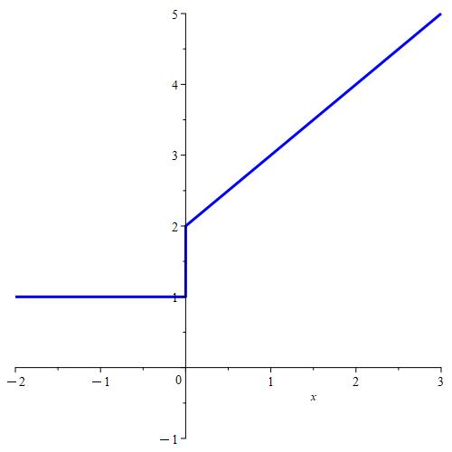
Figure 4: The graph of
has a vertical jump right at x = 0. Here, x = 0 is part of the constant piece where the function equals 1.
So far, we’ve only considered maxima or minima. Something else we may be concerned about (in later chapters, we definitely will be concerned about) whether or not a function passes through all of it’s intermediate values. For Problem 1, our function was y = 2x + 3. The domain’s boundary points were x = -1 and x = 2. The function’s range was bounded by y = 1 and y = 7 respectively. With this function on those intervals, there are x values that produce a value of y = 2, 3, 4, 5, and 6. There is even a value of x which produces a value of y = π ( this occurs at (x = (π – 3)/2).) For any value of y between 1 and 7, we can find a value of x that produces that value under the function.
Over those same intervals though, we could not guarantee that the function assumes the value of 8, 100, 1000, -500, or any other number not between 1 and 7.
For Problem 2, our function was y = x2 – x – 6. Even though the boundary points of the domain were 0 and 1, and the function’s values at those points were -6 and -4 respectively, we could still find x values that produce any value of y between -6 and -4. In this case, we could also find values of x that lead to values of y between -6.25 and -6.
These graphs did not have any weird behavior as did the function in Problem 3. Our next example explores this phenomenon a little bit more
The given function has a graph that splits off at x = 0. There is a big gap here as the function jumps from y = 1 to y = 2 abruptly.
a.)
For the interval (0, 2], we have that
f( (0, 2] ) = (2, 4]
Because 2 < 2.5 < 4, we expect we can find an x value such that f(x) = 2.5. Here, the only value that achieves that is x = 0.5.
Indeed, we see that f(0.5) = 2 + 0.5 = 2.5 as desired.
b.)
This function will take on every value in (2, 4] because we can easily solve the equation
y = 2 + x
for any value of y ∈ (2, 4].
c.)
Here, the function jumps from y = 1 at x = 0 to y > 2 for all x > 0. Hence, there is no value of x that will produce a value of y = 1.5.
We can go even farther and say that no value of x will produce a y value anywhere in the interval (1, 2]. Remember that f(0) = 1, and not 2.
At this point we’ve seen several examples of how including or excluding boundary points of an input interval impacts whether or not maxima or minima are achieved, and whether or not all intermediate values of a function are achieved. We’ve also seen how a function’s behavior over any interval plays a role, though that will be examined starting in the next chapter.
In this chapter, we take a closer look at the properties of these open and closed intervals.