Physical Address
304 North Cardinal St.
Dorchester Center, MA 02124
Now that we have a handle on what open and closed sets are within ℝ, we can start to elucidate more of their properties. In the previous section, we saw how to build up open sets from smaller open sets. Here, we’ll see a way to decompose open sets. We’ll also flesh out a property of every neighborhood centered at some limit point. We’ll see that this property gives rise to a new definition of limit point that is equivalent to the two definitions we’ve already seen.
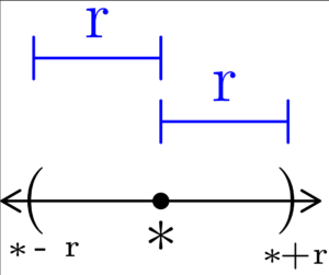
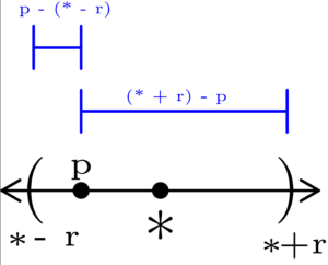
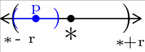
Figure 1: To show that a neighborhood is open, we can show that each point of a neighborhood is an interior point of that neighborhood. In (a), we start with an arbitrary neighborhood centered at ✻ with radius r. In (b), we select an arbitrary point p in the neighborhood of ✻, and note p’s distance from the neighborhood’s endpoints. In (c), we form a neighborhood centered at p with the smaller of the two distances found in (b). This gives us a neighborhood we need to show that p is an interior point of ✻’s neighborhood.
In the section on open sets, we intuitively described why any set of the form (a, b) is an open set. Here, we are going to be more exact in our description, and provide a formal proof of the fact. Using the language of neighborhoods from our discussion of metric spaces, we see that for ℝ, and any point p ∈ ℝ, we have that
Nr(p) = {q | q ∈ ℝ ∧ d(p, q) < r} = (p – r, p + r) = (a, b)
where a = p – r, and b = p + r.
Every neighborhood N ⊆ ℝ is an open set.
General Strategy: We simply pick an arbitrary point within a neighborhood, and show that it also a neighborhood contained entirely within the outer neighborhood. We do this by picking a radius small enough to be contained within the neighborhood.
Just to be somewhat whimsical, let ✻ ∈ ℝ be the center of neighborhood N with radius r so that
Nr(✻) = (✻ – r, ✻ + r) ⊆ ℝ.
Now, let p ∈ Nr(✻), meaning p ∈ (✻ – r, ✻ + r). Letting
r’ = min( p – (✻ – r), (✻ + r) – p )
gives us a neighborhood Nr’(p) such that
Nr’(p) ⊆ Nr(✻).
Meaning that for the arbitrarily picked point p, we found a neighborhood centered at p that is entirely contained within Nr(✻). This means that p is an interior point of Nr(✻), and since it was arbitrarily picked, we must have that every point within Nr(✻) is an interior point of Nr(✻).
Thus by definition, Nr(✻). is an open. Finally noting that Nr(✻) was itself an arbitrarily picked neighborhood of ℝ, we have that every neighborhood of ℝ must be an open set as desired.
After spending some amount of time trying to come up with examples of open subsets of ℝ, you may start thinking that all such sets are of the form (a, b), or unions of such sets. One of the open subsets may be of the form (-∞, a), and may also include an interval of the form (b, ∞). The next theorem establishes this observation as a fact. Though the theorem is simple to state and seems obvious after a little bit of thought, there are some subtle pints to iron out.
Every open set E ⊆ ℝ is a countable union of disjoint open intervals.
General Strategy: For each point in the open set, we construct it’s largest containing subset within the open set. We form a partition of the neighborhood using these constructed intervals, and then finally show that they are countable by putting them in a bijection with a subset of ℚ. For this proof, we’ll break it down into the same 3 steps.
Step 1: For any point x ∈ E, find the largest subset of E containing x
Let E ⊆ ℝ be an open set, and let x ∈ E.
By definition then, there exists some r > 0 such that
Nr(x) = (x – r, x + r) ⊆ E
Let Ix = (αx, βx) where
αx = inf( {a : (a, x) ⊆ E} )
βx = sup({b : (x, b) ⊆ E} )
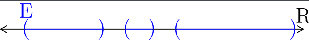
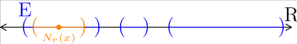
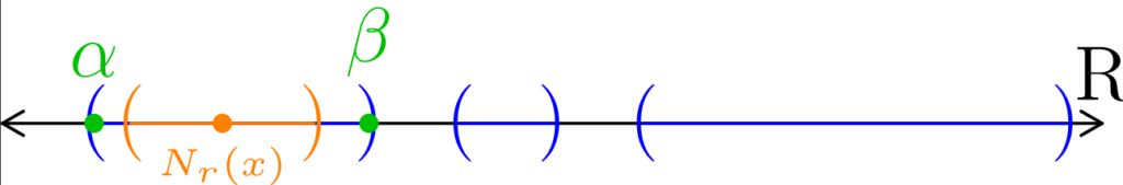

Figure 2: In (a), we show an example of an open set (colored blue) E within ℝ. As depicted in (b), we first pick some point x in the open set (colored orange) and form a neighborhood with radius r centered at x so it is entirely contained within E. We also color the neighborhood orange. You’ll notice that the chosen neighborhood is not the largest subset of E containing x. In (c), we note that the set (α, β) – with the endpoints colored green – is the largest subset of E containing x. Finally in (d), we give that largest set the name Ix, which is again colored green for clarity.
Thus, Ix is the largest open interval containing x such that
Ix ⊆ E
Step 2: Show that these largest subsets form a partition of E
Now, suppose y ∈ E such that x < y (the situation where y < x is analogous.)
Let αy, βy, and Iy be defined analogously to αx, βx, and Ix respectively.
If Ix ∩ Iy ≠ ∅, then for any z ∈ Ix ∩ Iy, we have that
αx < z < βx
Note that because Ix and Iy are both subsets of ✻, and because z ∈ Ix ∩ Iy, we also have that z ∈ E.
Furthermore,
(αx, z) ⊆ Ix ⇒ (αx, z) ⊆ E
(z, y) ⊆ Iy ⇒ (z, y) ⊆ E
This means that
(αx, z) ∪ {z} ∪ (z, y) ⊆ E
and since αx is the infimum of Ix, αx must also be the infimum of Iy (remember that Iy is defined as
αy = inf( {a : (a, y) ⊆ E} )
βy = sup({b : (y, b) ⊆ E} )
Iy = (αy, βy)
which is the largest open interval containing y that is a subset of E.)
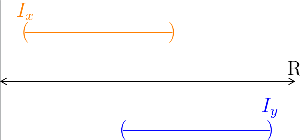
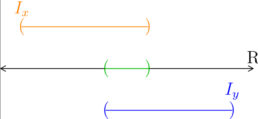
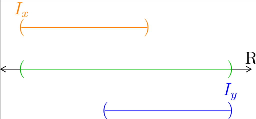
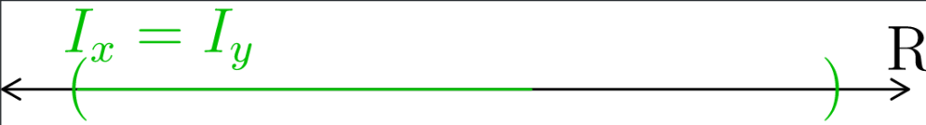
Figure 3: Here, we demonstrate why if Ix (colored orange) and Iy (colored blue) have any amount of overlap, then they must actually be the same set (using the terminology of partitions and equivalence relations, we’d say they represent the same class.) In (a), we show two intervals that have a non-empty intersection. In (b), we show the intersection explicitly in green. Notice that the points that are in the green interval are also in an interval whose infimum is the infimum of Ix, and are also in an interval whose supremum is the same as that of Iy. Thus, as depicted, neither Ix nor Iy is the largest interval containing the green points. In (c), we extend the green interval to be as large as possible. In (d), we recognize that Ix and Iy would actually refer to the large green interval. Neither the orange or blue intervals depicted in (a) – (c) were actually Ix and Iy because they were actually not the largest intervals containing those points.
For analogous reasons, sup(Iy) = sup(Ix). This means that Ix = Iy.
Thus, all open intervals of the form Ix, constructed by taking points in E not already in some other open interval Iy, will form a partition of E.
Now we have a way of partitioning any open set in ℝ into open intervals.
Step 3: Show that the partition has a countable number of open intervals
In each open interval Ix of the partition of E, there will be some rational number qx ∈ Ix. This is guaranteed because of the density of ℚ in ℝ.
We thus associate to each open interval Ix of the partition of E the number qx using the bijective function
f(Ix) = qx.
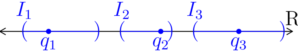
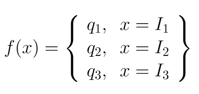
Figure 4: Because ℚ is dense in ℝ, in any open interval of ℝ exists some rational number q. In (a), we use the density of ℚ in ℝ to pick some rational number in each of the open intervals constructed from step 2 of this proof. In (b), we explicitly show the bijection from each interval to the rational number chosen within that interval. Because such a bijection exists, we can essentially label each open interval with a rational number.
Because ℚ is countable, every subset of ℚ is also countable, and since we’ve just formed a bijection between the partition of E with a subset of ℚ, that means that there are a countable number of open intervals in the partition of E.
Thus, we’ve found a way to partition an arbitrarily chosen open subset E of ℝ into a countable number of open intervals. This means that any open subset of ℝ is a countable union of disjoint open intervals as desired.
Figure 5: Consider the orange point at (1, 0). Here, we show some of the points from the sequence {1 / n}. As long as they are in the neighborhood, those points are colored green. When they’re not in the neighborhood, they become red. Notice that once the closest point to (1, 0) is outside the neighborhood, no other neighborhood intersects the sequence. Hence, the orange point can’t be a limit point for the sequence {1 / n}.
If p is a limit point for some set E ⊆ ℝ, then every neighborhood of p contains infinitely many points from E.
General Strategy: Assuming that this is not true will lead to a contradiction. If there is a neighborhood with a finite amount of points from E, then a neighborhood can be constructed that does not intersect E anywhere other than p. This contradicts p being a limit point for E.
Presume – for the purpose of showing a contradiction – that p is a limit point for E that has a neighborhood N with radius r having only a finite number of points from E.
Because there are finitely many points in Nr(p), we can label them
p1, p2, p3, p4, … , pn.
Because p is in it’s own neighborhood, we must have that n ≥ 1. Note that we don’t necessarily need p ∈ E. We just need p to be a limit point for E.
Suppose n = 1, then Nr(p) = {p} ⊈ E \ {p}, contradicting the fact that p is a limit point for E.
Suppose n > 1, then let q ≠ p be the point in Nr(p) that is closest to p (we can do this since there are finitely many points within the neighborhood.) Define r’ = d(p, q).
Then
Nr’(p) ∩ E \ {p} = ∅
again contradicting the fact that p is a limit point for E (because we found a neighborhood centered at p that does not intersect E at any point other than p.)
Either way, if any neighborhood of p intersects E only at a finite number of points, then there exists a neighborhood centered at p that does not intersect E at any other point except possibly at p itself. Thus, p can’t be a limit point of E. This contradicts the fact that p is a limit for E.
Thus, it must be the case that if p is a limit point for E, then every neighborhood must intersect E at infinitely many points (since it intersects E at infinitely many points, we don’t care if p is one of those points, there are infinitely many others.)
Figure 6: Here, we consider the open set (0, 1.1). 0 is a limit point for this interval. We start with a neighborhood of radius 1.1 centered at 0, and use 1 (colored green) as the first point in our sequence. Once the radius is smaller than 1, we pick the point 1/2 (colored green.) Once the radius is smaller than 1/2, we pick a new point (1/3 in this example), and every time the radius is smaller than the most recently chosen point, we pick yet another point within the orange neighborhood. For all r > 0, we can keep doing this process to construct an infinite sequence that converges to 0.
Suppose E ⊆ ℝ and that p is a limit point for E. We can use the same reasoning used in the proof for Theorem 3 to build a sequence of points within E \ {p} that converges to p.
The construction of such a sequence starts by picking any r1 > 0, and then picking some point p1 ∈ Nr1(p) \ {p} ∩ E. The point p1 ∈ E will be the first point of the sequence.
Next, we let r2 = |p – p1|. We can then pick a point p2 from Nr2(p) \ {p} ∩ E. Note that p1 ∉ Nr2(p) \ {p} because of how r2 was defined. Specifically, we have that r2 = |p – p1| < r1, hence p1 is more than r2 away from p. Now we have the points
{p1, p2} ⊆ E \ {p}.
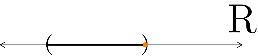
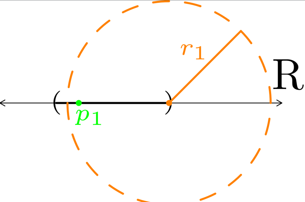
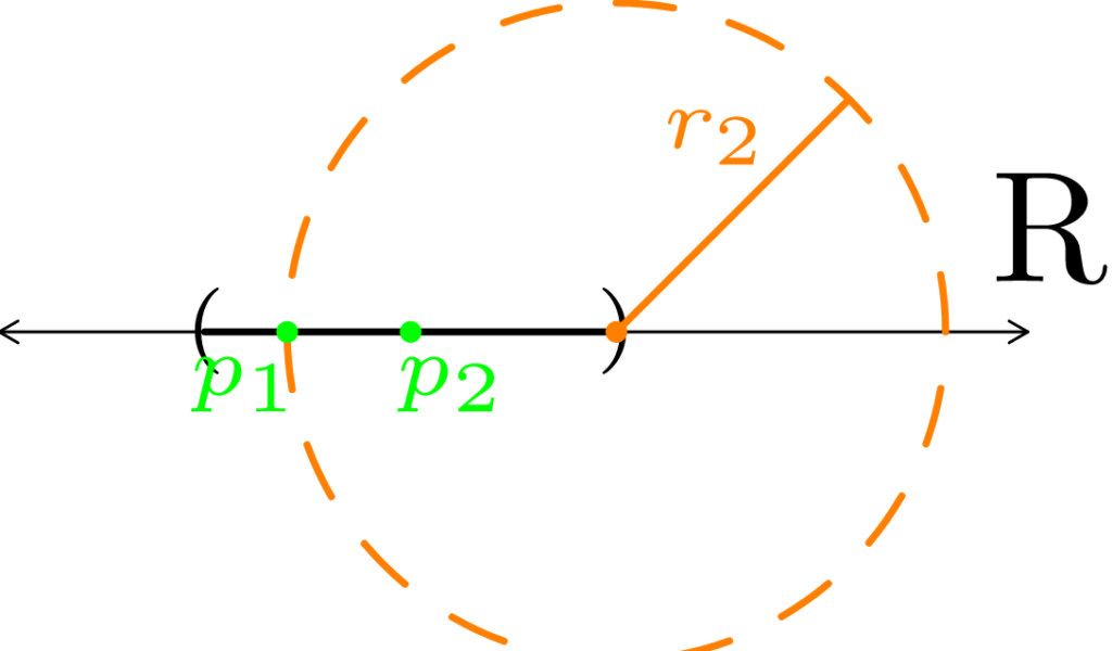
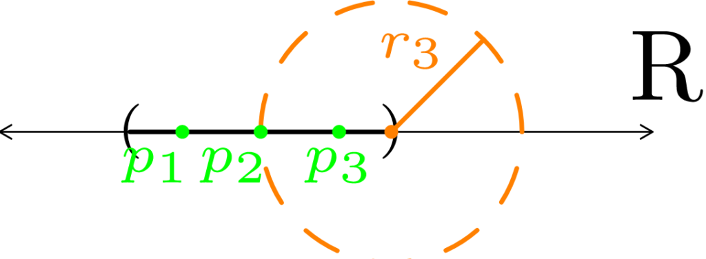
Figure 7: In (a), we start with an open interval within ℝ. We choose a the right boundary point as our limit point (colored orange) to use in constructing a convergent sequence. In (b), we pick r1 > 0, and pick a point p1 that is within both the orange neighborhood and in the open interval. In (c), we make our new radius r2 based on how far away p1 is from the orange point. We then pick a new point within the orange neighborhood and call it p2. In (d), we repeat what we did in (b) and (c) to get a new radius r3 and a new point p3. As demonstrated in Figure 6, this process can continue infinitely long to produce a sequence within the open interval that converges to the orange point.
The logic also works the other way. If we had a sequence of points in E \ {p} that converges to p, then p must be a limit point for E. Because there is an infinite sequence of points converging to p, there are infinitely many neighborhoods of p intersecting E at some point other than p itself.
Based on the fact that limit points imply the existence of some sequence within E converging to p, and that the existence of a sequence in E converging to p implies that p is a limit point of E, we have a new definition of limit point that is equivalent to the other definitions of limit point we’ve seen so far.
Let E ⊆ ℝ.
A point p ∈ ℝ is a limit point of E if there exists some sequence of points
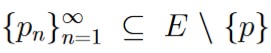
that converges to p.
A finite point set has no limit points.
Suppose E was a finite point set within ℝ. If there were any limit points of E, then every neighborhood of that limit point would intersect E at infinitely many points. This is impossible for a finite point set, hence there can be no limit points for E as desired.