Physical Address
304 North Cardinal St.
Dorchester Center, MA 02124
After taking into account all requirements imposed by the axioms, there are still infinitely many valid probability functions that can be taken. We saw this when interpreting the axioms in this section. Even for an experiment as simple as flipping a coin, there are infinitely many ways to assign probabilities to heads and tails.
For any experiment, unless we’re specifically told how often some event occurs relative to the other events, then we don’t know the experiment’s probability function. However, for many experiments, there is no reason to assume that any one point within the sample space is any more likely to occur than any other point. Consider the flip of a coin. Unless we’re told otherwise, there is no reason to assume that heads is more likely to show than tails. In other words, unless we’re specifically told the coin has a bias, we should assume that the probability of landing heads is equal to the probability of landing tails.
This is the same situation with a die. Unless otherwise told, there is no reason to assume that any one side is more likely to show up than any other side. Typically, we just assume that all sides are equally likely to appear.
The assumption that all points from the sample space are equally likely is often a key assumption in many probability problems. This assumption, combined with all of the theorems in the previous sections, gives us the ability to solve many problems.
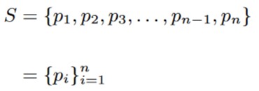
Suppose for some experiment, we have a sample space S with n points:
The assumption of uniform randomness gives us the following:

Now, we combine this assumption with Axiom 2 and Theorem 1.4.2 to get the following:
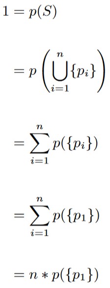
Based on this we get that
p({p1}) = 1/n.
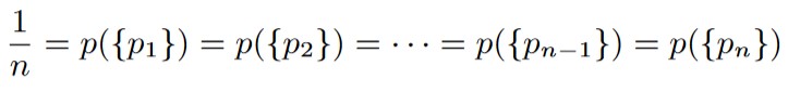
Furthermore, because of our assumption of uniform randomness, we also have that
This is the basic strategy we’ll use for multiple types of experiments with discrete outcomes.
We saw from Example 1.3.3 how to calculate the probability that a coin lands heads up when we know the coin’s bias. This time, let’s use the assumption of uniform randomness; that is to say; let’s assume that it is equally likely that the coin will land heads up as it will land tails up. We also make use of Theorem 1.4.2 and Axiom 2.
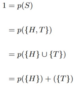
With the assumption of uniform randomness, we assume that
p({H}) = p({T}).
Now, we make the substitution in order to solve. for the probabilities.
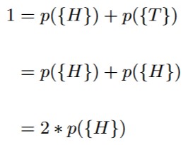
This tells us that
p({H}) = 1/2,
and since p({T}) = p({H}), we also have that p({T}) = 1/2 as well.
| First Flip \ Second Flip | H | T |
| H | HH | HT |
| T | TH | TT |
Figure 1.5.1: The sample space for flipping a coin twice involves recording the first flip and the second flip. Here, we show the sample space in a tabular format.
Now let’s consider an experiment where we flip a coin twice. The first thing we do is clearly specify the sample space. Since we’re flipping a coin twice, we need to record the result of the first flip, and the second flip. Instead of using ordered pairs, we’ll just list the results back to back:
S = {HH, HT, TH, TT}.
Under the assumption of uniform randomness, we have that
p({HH}) = p({HT}) = p({TH}) = p({TT}).
Combining this assumption with Axiom 2 and Theorem 1.4.2 gives us the following:
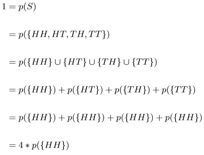
This tells us that p({HH}) = 1/4. Now that we know p({HH}), we now know the probabilities of the other points from the sample space:
1/4 = p({HH}) = p({HT}) = p({TH}) = p({TT}).
Now that we know the individual probabilities of each point within the sample space, we’re ready to solve problems.
Consider an experiment where you flip a coin twice. What’s the probability that tails shows up no more than once?
To answer this question, let’s clearly define what event we want. We’re told that tails shows up no more than once. That means it can show up 0 times, or 1 time. Looking at the table from Figure 1.5.1, let’s color all cells where this condition is met green:
| HH | HT |
| TH | TT |
| HH | HT |
| TH | TT |
Based on this, we see that the event we’re interested in is
E = {HH, HT, TH}.
Invoking Theorem 1.4.2, we get that
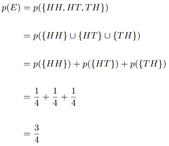
Thus, we get that the probability of the event
E = “Tails shows up no more than once”
is 3/4. As a percentage, this is 75%.
Consider an experiment where you are flipping a coin twice. What’s the probability that both flips are the same?
Again, we start by clearly defining what the event is. Instead of drawing the tables again, we just list what points from the sample space satisfy the condition:
E = {HH, TT}.
Now, we invoke Theorem 1.4.2 just as we did in example 1.5.1:
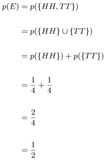
And so, the probability that both flips result in the same outcome is 1/2, or 50%.
Consider an experiment where you flip a coin twice. What’s the probability that the first flip is different than the second flip?
Here, we’ll actually make use of Theorem 1.4.3, which relates the probability of an event to the probability of that event’s complementary event. Notice the event we’re interested in is
E = {HT, TH}.
The complement of this event is
EC = {HH, TT}.
From Example 1.5.2, we know that p(EC) = 1/2. Thus, by invoking Theorem 1.4.3, we get that
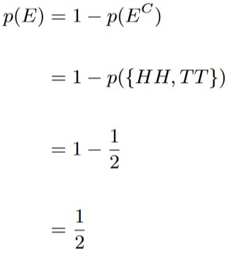
So p({HT, TH}) = 1/2.
Just as we did with a single coin, we can start by using the assumption of uniform randomness to calculate the probability of any one face on a six-sided dice showing up. First, as always, we clearly define the sample space:
S = {1, 2, 3, 4, 5, 6}.
Now, the assumption of uniform randomness tells us that each point within the sample space is equally likely:
p({1}) = p({2}) = p({3}) = p({4}) = p({5}) = p({6}).
Now we invoke Axiom 2 and Theorem 1.4.2 just as we did with the coin experiment:
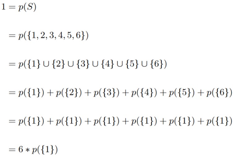
This tells us that p({1}) = 1/6. From this, we get the following:
1/6 = p({1}) + p({2}) + p({3}) + p({4}) + p({5}) + p({6}).
| Die 1 \ Die 2 | 1 | 2 | 3 | 4 | 5 | 6 |
| 1 | (1, 1) | (1, 2) | (1, 3) | (1, 4) | (1, 5) | (1, 6) |
| 2 | (2, 1) | (2, 2) | (2, 3) | (2, 4) | (2, 5) | (2, 6) |
| 3 | (3, 1) | (3, 2) | (3, 3) | (3, 4) | (3, 5) | (3, 6) |
| 4 | (4, 1) | (4, 2) | (4, 3) | (4, 4) | (4, 5) | (4, 6) |
| 5 | (5, 1) | (5, 2) | (5, 3) | (5, 4) | (5, 5) | (5, 6) |
| 6 | (6, 1) | (6, 2) | (6, 3) | (6, 4) | (6, 5) | (6, 6) |
(a)
| Die 1 \ Die 2 | 1 | 2 | 3 | 4 | 5 | 6 |
| 1 | 2 | 3 | 4 | 5 | 6 | 7 |
| 2 | 3 | 4 | 5 | 6 | 7 | 8 |
| 3 | 4 | 5 | 6 | 7 | 8 | 9 |
| 4 | 5 | 6 | 7 | 8 | 9 | 10 |
| 5 | 6 | 7 | 8 | 9 | 10 | 11 |
| 6 | 7 | 8 | 9 | 10 | 11 | 12 |
(b)
Figure 1.5.2: Since each die is unaffected by the other die, there are 6 * 6 = 36 total points within the sample space. Here, each point is the form of an ordered pair
(Die #1, Die #2).
In (a), we simply show the points in the sample space. In (b), we show the sum of the rolls.
Now consider the experiment of rolling two dice. The sample space for this experiment is shown in Figure 1.5.2. Since the results of one of the die does not in any way affect the outcome of the other die, there are 6 * 6 = 36 total elements within the sample space. Under the assumption of uniform randomness, each of the 36 outcomes is equally likely. This gives us that
p((1, 1)) = p((1, 2)) = p((1, 3)) = … = p((6, 4)) = p((6, 5)) = p((6, 6)).
Using the exact same logic from the coin calculations, we get that
1/36 = p((1, 1)) = p((1, 2)) = p((1, 3)) = … = p((6, 4)) = p((6, 5)) = p((6, 6)).
Consider the experiment of rolling two dice. What’s the probability that either number rolled is a prime number?
As always, we start by clearly specifying the event of interest. Here, we’ll copy the table from part (a) of Figure 1.5.2, and color all cells with appropriate outcomes green.
| Die 1 \ Die 2 | 1 | 2 | 3 | 4 | 5 | 6 |
| 1 | (1, 1) | (1, 2) | (1, 3) | (1, 4) | (1, 5) | (1, 6) |
| 2 | (2, 1) | (2, 2) | (2, 3) | (2, 4) | (2, 5) | (2, 6) |
| 3 | (3, 1) | (3, 2) | (3, 3) | (3, 4) | (3, 5) | (3, 6) |
| 4 | (4, 1) | (4, 2) | (4, 3) | (4, 4) | (4, 5) | (4, 6) |
| 5 | (5, 1) | (5, 2) | (5, 3) | (5, 4) | (5, 5) | (5, 6) |
| 6 | (6, 1) | (6, 2) | (6, 3) | (6, 4) | (6, 5) | (6, 6) |
We can count the number of points satisfying the condition, which is 27. This means that to calculate the probability, we have to add together the probability of 27 of the points from the sample space. Hence,
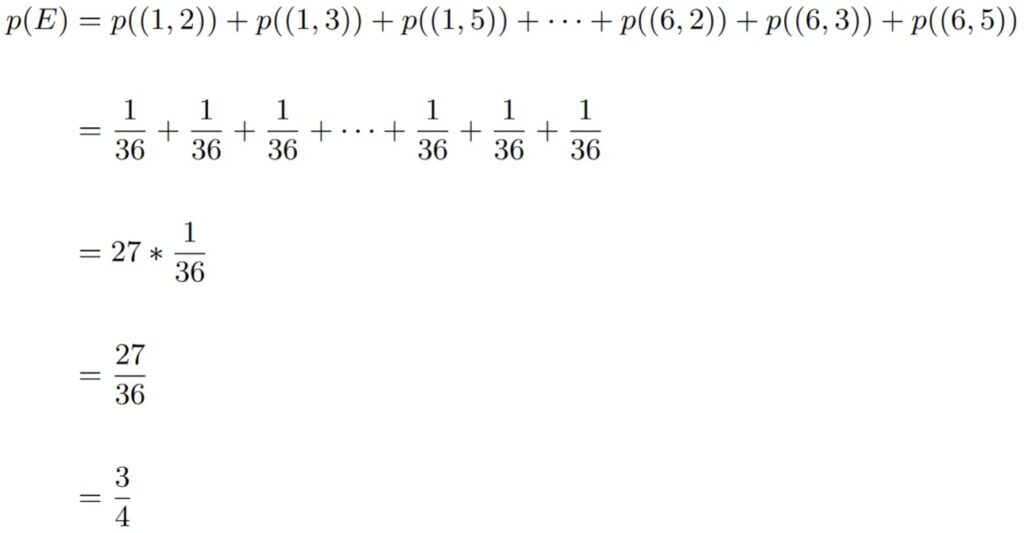
So, the probability of event
E = “Either roll is a prime number”
occurring is 3/4.
Consider the experiment of rolling two dice. What’s the probability that the sum of the two rolls is 7?
We’re looking for points from the sample space that yield a sum of 7. According to the table in (b) from Figure 1.5.2, the event we’re interested in is the following:
E = {(1, 6), (2, 5), (3, 4), (4, 3), (5, 2), (6, 1)}.
Because we know that the probability of each of these individual points is 1/36, we get the following:
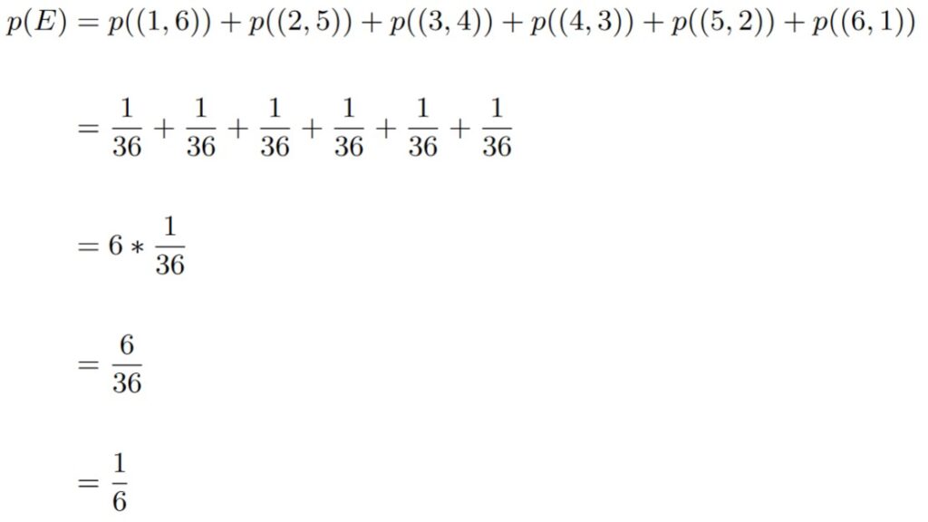
So the probability of rolling a sum of 7 is 1/6.
Consider the experiment of rolling two dice. What’s the probability that both rolls are prime numbers?
Here, the event we’re interested in is the event
E = {2, 3, 5} ✕ {2, 3, 5}.
There are 9 such points in the event, all with probability 1/36 of occurring. This tells us that the probability of both rolls being prime is
p(E) = 9 * 1/36 = 9/36 = 1/4.
Consider the experiment of rolling two dice. What’s the probability that only one of the rolls is a prime number?
Notice that this event is basically what results when we take the event
B = “Either number rolled is a prime number”
from Example 1.5.4 and take remove the elements of the event
A = “Both numbers rolled are prime”
from Example 1.5.6. In other words, the event E we’re interested in is
E = B – A,
and since A ⊆ B, we can invoke Theorem 1.4.4 as follows:
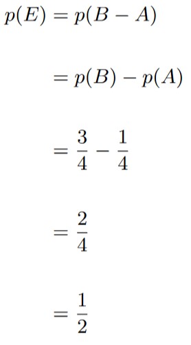
So the probability that only one of the rolls is prime is 1/2.
We need to be careful to not assume uniform randomness when such an assumption is not warranted.
One example of such an error can occur when we roll two dice and observe their sum. Let’s take a look at the sample space for this experiment:
S = {2, 3, 4, 5, 6, 7,8 9, 10, 11, 12}.
Notice that |S| = 11. If we were to assume uniform randomness, we’d have that
1/11 = p({2}) = p({3}) = p({4}) = p({5}) = p({6}) = p({7}) = p({8}) = p({9}) = p({10}) = p({11}) = p({12}).
Past experience with various dice games may lead us to not accept the above probabilities. For instance, above we see that with the assumption of uniform randomness, the sums 2 and 12 are just as likely to show up as a sum of 7. This seems like an outrageous claim, but it is the correct claim when uniform randomness is assumed.
The problem is that rolling a sum of 3 is twice as likely to occur as a sum of 2. This is because when two dice are rolled, there are two ways to make a sum of 3:
“3” = {(1, 2), (2, 1)},
as opposed to rolling a sum of 2, which can only occur in one way:
“2” = {(1, 1)}.
To help avoid this issue, it’s best to record all relevant information. If you roll two dice, record the results of both rolls, not just some combination of the two rolls. For flipping coins, record the outcome for each coin, don’t just record a single number that captures all information form the coins.
In short, if you conduct an experiment that involves multiple objects, record the result from each object.