The Axioms of Probability

Now that we know how to describe events from a sample space, we need to start formulating the likelihood of some event occurring during an experiment that involves random chance. That is to say, we need to start figuring out what the probability for event is.

Just like in any other branch of math, we start with a few axioms. Those axioms yield theorems that can make our calculations easier, or give us more insight into the problem at hand. For probability, the axioms we take were conceived by Andrey Kolmogorov in 1933 with the publication of his book “Foundations of the Theory of Probability.”

To understand these axioms, we first develop the notion of a probability function.

Probability Functions

In essence, what we’re trying to do when calculating a probability is to take some event E with a sample space S, and assign some number to it.

Example 1.3.1

Suppose we want to calculate the probability that a coin flip results in a “Heads” outcome. Intuitively, we want to say that the probability of such an outcome is 1/2, or we may even want to say 50%.

We could extend this to other events. Let’s recall the sample space of flipping a coin once, ignoring the possibility of landing on the side:

S = {H, T}

There are a total of 4 events that can occur:

∅	–	The event where nothing happens
{H}	–	The event where the coin lands heads
{T}	–	The event where the coin lands tails
{H, T}	–	The event where the coin lands heads or tails

Notice that the above 4 events, when combined into a set, is simply the power set of the sample space.

We can define a function, which we’ll denote p.

p(∅) = 0	If you flip a coin, it will land on a side, so this event can’t possibly occur.
p( {H} ) = 1/2	We expect that, half of the time, the coin will land heads.
p( {T} ) = 1/2	We expect that, half of the time, the coin will land tails.
p( {H, T} ) = 1	The coin will land on one if its sides, so this event captures all possible outcomes.

What about the possibility of landing heads and tails? In a single coin flip, this scenario is impossible, so it doesn’t make sense to define a probability for it. It only makes sense to define a probability on subsets of the sample space.

In the above example, we noted that any subset of the experiment’s sample space can be assigned a probability. However, any set that is not a subset of a sample space can’t meaningfully be assigned a probability. Additionally, in all scenarios, the probability assigned to each event was a real number. We call the real number assigned to each event by the function the probability of that event.

Probability Function, Probability

Consider an experiment with sample space S.

The probability function of the experiment, denoted p, is the function that assigns to each event from the sample space (each element of the sample space’s power set) a real number from ℝ. Symbolically, we write

p: P(S) → ℝ.

The number x ∈ ℝ that is assigned to an event E ∈ P(S) by p is called the probability of E, and we write

p(E) = x.

The Axioms

The axioms for probability are essentially imposed conditions on probability functions. There are three such axioms.

The Axioms of Probability

Consider an experiment with sample space S.

Non-negativity: For any event E within the sample space S, p(E) ≥ 0.
Probability of the Sample Space: p(S) = 1.
Additivity: For any set of mutually exclusive events {E₁, E₂, E₃, …},

Let’s discuss these axioms one at a time.

Axiom 1: Non-negativity

All this axiom says is that a probability should be non-negative, which should make some intuitive sense. What would it mean for an event to have negative probability? What does an event having a -50% chance probability of happening mean? The idea of a negative probability is nonsensical, and this axiom just asserts that for a function to be a probability function, it must be non-negative.

Axiom 2: Probability of the Sample Space

In essence, the probability of any outcome occurring within the sample space is 1. Thus, if you examine the sample space, one of its members will always be the outcome of the underlying experiment. Take the coin flip example from Example 1.3.1. If we flip a coin, it will always land either Heads or Tails. Thus, p({H, T}) = p(S) = 1.

The number chosen did not have to be 1. For example, we could have taken the number 100, and then we could interpret probabilities as percentages. The number 1 is used because it is simple.

Axiom 3: Additivity

This axiom simply states that if you have mutually exclusive events, then the probability of any of the events occurring is the sum of their individual probabilities. Let’s look at an example.

Example 1.3.2

Consider the experiment of drawing a card from a well-shuffled deck.

Let’s take a look at the entire sample space.

♠

🂡

🂢

🂣

🂤

🂥

🂦

🂧

🂨

🂩

🂫

🂭

🂮

♣

🃑

🃒

🃓

🃔

🃕

🃖

🃗

🃘

🃙

🃚

🃛

🃝

🃞

♦

🃁

🃂

🃃

🃄

🃅

🃆

🃇

🃈

🃉

🃊

🃋

🃍

🃎

♥

🂱

🂲

🂳

🂴

🂵

🂶

🂷

🂸

🂹

🂺

🂻

🂽

🂾

Lets specify a couple of events for this sample space.

R: “Draw a red card”
B: “Draw a black card”

Here, R is mutually exclusive to B since no card is both red and black. Hence, according to axiom 3, we have that

p({R} ∪ {B}) = p({R}) + p({B}).

Now consider the two following events.

D: “Draw a diamond”
J: “Draw a jack”

Notice that events D and J are not mutually exclusive since (♦, J) belongs to both events. Thus, we can’t appeal to Axiom 3 to conclude that

p({D} ∪ {J}) = p({D}) + p({J}).

Instead, we’ll need other methods to deal with this event.

Interpreting the Axioms

The axioms give us a way to start calculating probabilities. To illustrate this, we’ll consider the experiment of flipping a coin. We’ll use the axioms to try and calculate the probability of getting heads, and the probability of getting tails.

As previously discussed, the sample space of this experiment is {H, T}, so there are only two outcomes. This means we only have two probabilities to calculate, those being p(H) and p(T). Suppose we could pick any values for p(H) and p(T) we wanted. Here are five such choices.

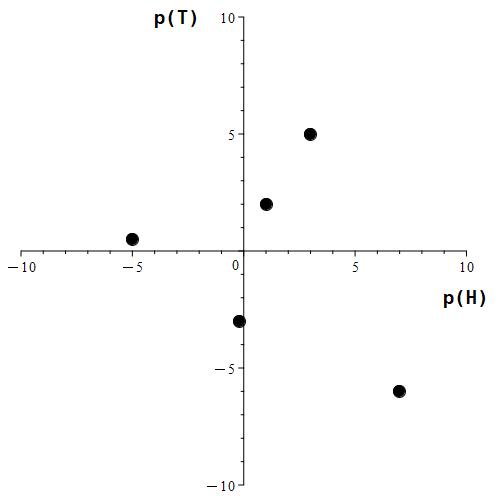
Figure 1.3.1: Here, we pick 5 values for p(H) and p(T). Notice that none of the values chosen for either p(H) or p(T) satisfy all axioms required for a probability. Some of the values chosen are even negative!

As demonstrated in Figure 1.3.1, picking values for p(H) and p(T) arbitrarily leads to nonsensical values. One of the chosen points is at (-0.2, -3), which according to the axis labels means that we have chosen p(H) = -0.2 and p(T) = -3. These values don’t make any intuitive sense when regarded as probabilities, which is what we’re trying to do. This is where the axioms come in.

The axioms impose conditions on what the probabilities of each event can be. The following figure demonstrates the effect of each axiom on what kinds of values can be selected for p(H) and p(T).

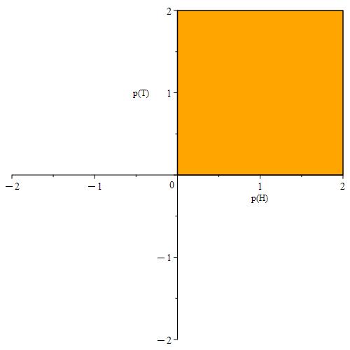
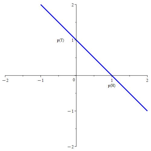
Figure 1.3.2: In (a), we plot all points (p(H), p(T)) where p(H) ≥ 0 and p(T) ≥ 0. This satisfies Axiom 1. In (b), we show an implicit plot where p(H) + p(T) = 1. This satisfies both Axioms 2 and 3.

Plot (a) from Figure 1.3.2 shows what points (p(H), p(T)) satisfy the requirement that p(H) ≥ 0 and p(T) ≥ 0, shown in orange. This is required by Axiom 1. In (b), we plot all points (p(H), p(T)) such that

p(H) + p(T) = 1,

shown in blue. Any points not on the line do not meet the requirements of Axiom 2. In a sense, the requirements of Axiom 3 are implicitly imposed within plot (b) of Figure 1.3.2 because Axiom 3 allows us to express p(S) like so:

p(S) = p({H, T}) = p({H} ∪ {T}) = p({H}) + p({T}) = 1.

We want to examine points that satisfy all three Axioms. Hence, we essentially need to know where the orange square and blue line segment intersect.

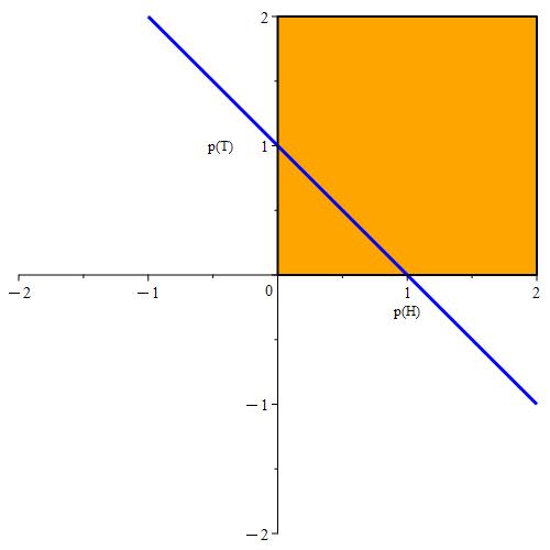
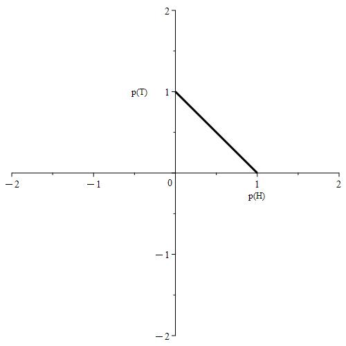
Figure 1.3.4: In (a), we combine all the plots from Figure 1.3.2 into one plot in order to see where the intersection lies. Both plots intersect at a line segment from (1, 0) to (0, 1). In (b), we just plot the line segment where the intersection occurs.

Notice that even after imposing all 3 Axioms, we still have infinitely many points that could represent the probabilities for p(H) and p(T). For example. the point (0.3, 0.7) is on this segment, which corresponds to the situation where p(H) = 0.3 and p(T) = 0.7. In this scenario, we would interpret this coin as being biased in favor of tails where tails comes up 70% of the time. However, the point (0.5, 0.5) is also on this segment, which corresponds to the situation where p(H) = 0.5 and p(T) = 0.5. Here, we have a fair coin where heads comes up 50% of the time, as does tails.

Because all of these points satisfy the axioms, all values are correct. If we want to have exactly one correct assignment for p(H) and p(T), we need an additional assumption. We would have to know the coin’s bias.

Example 1.3.3

Suppose we knew that a certain coin came up heads twice as often as tails; in other words,

p(H) = 2 * p(T).

We could combine this observation with the fact that

p(H) + p(T) = 1

to figure out what both p(H) and p(T) have to be. Basically, we have a system of two equations with two unknowns.

	p(H) + p(T) = 1
⟹	2*p(T) + p(T) = 1
⟹	3*p(T) = 1
⟹	p(T) = 1/3

Now that we know that p(T) = 1/3, and because p(H) = 2*p(T), we also have that

p(H) = 2*p(T) = 2*(1/3) = 2/3.

So now we know that we’re dealing with such a coin that has an approximately 66.7% chance of coming up heads, and roughly a 33.3% chance of coming up tails.

Axiom 3 with Finite Events

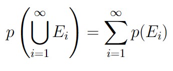
One last thing to note about Axiom 3 is that it was stated for an infinite number of events. Even so, we’ve been using it throughout this page on only a finite number of events, either dealing with drawing cards from a deck, or flipping a coin.

The reason we’ve been able to do this is the fact that the probability of the null event ∅ is always 0 (proven in the next section.) For our coin example, we could note that for an infinite number of events

{E₁, E₂, E₃, E₄, …},

let

H = E₁,
T = E₂,
∅ = E₃ = E₄ = E₅ = …

Now we can invoke Axiom 3 as normal, and carry out some basic algebra, as seen below.

Now our use of Axiom 3 on a finite number of event is at least somewhat justified. Again, the next section fully justifies such usage.