Sample Spaces and Events

Often when analyzing some experiment, we’ll want to know what kinds of results we can expect to observe. For instance, if we’re flipping a coin, we can expect the coin to either land heads up or tails up as long as we ignore the occurrence of landing on its side (though on occasion, we may also be interested in cases where the coin lands on its side.) If we’re rolling a single six-sided die, we can reasonably expect the die to land so that its 1-face, 2-face, 3-face, 4-face, 5-face, or 6-face is showing up. When dealing with a standard deck of playing cards, we can reasonably expect the card to be one of two colors, one of four suits, and one of thirteen values.

The experiments we consider don’t necessarily have to have discrete values either. When tossing a dart at a dartboard with radius 20 inches, we can measure the dart’s position using distance from the center as being any real number in the interval [0, 20], and we can measure the polar angle to be any real number in the interval [0, 2π). We can measure how often a certain airline manages to deliver planes for its customer within a five minute window of a promise time, we can measure how much time in minutes it takes for a bus to arrive at a predetermined stop after 12:00PM, we can measure how long in days it takes for a vending machine to go out of service, and so on.

Being able to articulate what set of possibilities exists for an experiment, and being able to describe a particular outcome of an experiment will often aid us in solving problems. In the parlance of probability, these sets and outcomes are referred to as sample spaces and events respectively.

Sample Spaces

Sample Space, Point

For a given experiment, the sample space is the set of all possible outcomes of the experiment. Usually, this kind of set is denoted S.

Each element within the experiment’s sample space is sometimes referred to as a point, or even as a sample point, of that sample space.

Example 1.1

Consider a first experiment of “Flipping a coin.” The sample space of this experiment, denoted S₁, would be the set

S₁ = {H, T}

where the letter H represents heads, and the letter T represents tails.

We could flip the coin twice, in which case we’d want to record the result of the first flip and the second flip. Using ordered pairs where the first element represents the first flip, and the second element represents the second flip, the associated sample space, denoted here as S₂, would be the set

S₂ = { (H, H), (H, T), (T, H), (T, T) }.

Alternatively, we could also just stick the letters side by side, in which case we would have the set

S₂ = { HH, HT, TH, TT }.

Example 1.2

For the experiment of rolling a six-sided die, the sample space would be

S₃ = { 1, 2, 3, 4, 5, 6 }.

We could roll the die twice, recording the results in an ordered pair similarly to what we did in example 1.1 in which case we would have the set

S₄ =	{	(1, 1), (1, 2), (1, 3), (1, 4), (1, 5), (1, 6),
		(2, 1), (2, 2), (2, 3), (2, 4), (2, 5), (2, 6),
		(3, 1), (3, 2), (3, 3), (3, 4), (3, 5), (3, 6),
		(4, 1), (4, 2), (4, 3), (4, 4), (4, 5), (4, 6),
		(5, 1), (5, 2), (5, 3), (5, 4), (5, 5), (5, 6),
		(6, 1), (6, 2), (6, 3), (6, 4), (6, 5), (6, 6)	}.

Since sample spaces are sets, we could use set operations to construct them. One way to write the sample space for the experiment of rolling a die twice above is to use a Cartesian Product and write

S₄ = {1, 2, 3, 4, 5, 6} ✕ {1, 2, 3, 4, 5, 6}

Example 1.3

For the experiment of drawing a card from a well-shuffled standard deck of playing cards, we could again use the Cartesian Product to describe the sample space as

S₅ = {♠, ♣, ♦, ♥} ✕ {A, 2, 3, 4, 5, 6, 7, 8, 9, 10, J, Q, K}

where the suits are enumerated in the first set, and in the second set we use A, J, Q, and K to represent the ace, jack, queen, and king respectively.

One point from this sample space would be the Ace of Spades (♠, A)

🂡.

A different sample point from this sample space would be the Three of Diamonds (♦, 3)

🃃.

Since there are 52 total cards in such a deck, the use of the Cartesian Product allows us to succinctly describe the sample space without having to list out every possibility.

Figure 1.1.1: We can interpret the sample space of Example 1.4 as a rectangle within ℝ². Along the x axis the the polar radius r of the dart. In the y direction we track the polar angle θ. Everything outside of the blue rectangle is not a point within the sample space.

Example 1.4

When dealing with an experiment with infinitely many outcomes, we must use some sort of set builder notation or Cartesian Product to define the experiment’s sample space.

Consider the experiment of throwing a dart at a dartboard with radius 20. We can use polar coordinates to measure the dart’s position. The polar radius will be any real number in the interval [0, 20]. The polar angle will be any real number in the interval [0, 2π). As such, we can’t simply list out all points in the sample space.

We could use set builder notation like this:

S₆ = { (r, θ) : 0 ≤ r ≤ 20 ∧ 0 ≤ θ < 2π}.

We could also use the Cartesian Product like this:

S₅ = [0, 20] ✕ [0, 2π)

Figure 1.1.2: For the experiment in Example 1.5, we can visualize the sample space as a collection of rays, each of which has their base at each non-negative integer point on the y-axis. Each ray extends infinitely to the right towards ∞.

Example 1.5

We can analyze experiments where the sample space is part finite (or countable) and part uncountably infinite.

Consider an experiment where for a particular arcade machine we want to record how many quarters it has received (a natural number or 0) and the time in minutes (a non-negative real number) it went out of service after being turned on.

In this case, we can use the Cartesian Product to define the sample space for this experiment as

S₇ = (ℕ ∪ {0}) ✕ (ℝ⁺ ∪ {0}).

Suppose for the arcade machine Space Blaster we record the sample point (123, 7200.3), meaning this machine has accepted 123 quarters ($30.75), and went out of service after being on for 7200.3 minutes (5 days and 18 minutes.) This equates to an income of 0.017 quarters per minute for this particular machine, or roughly 1 quarter per hour. Perhaps Space Blaster is not a very popular game.

On the other hand, suppose for the arcade machine Karate Chop we record the point (987, 11107.2). Karate Chop collected 987 quarters ($246.75), and went out of service after being on for 11107.2 minutes (7 days, 17 hours, 7 minutes, and 12 seconds.) This equates to a rate of 0.089 quarters per minute, or roughly 5 quarters every hour.

Events

Now that we have a way of characterizing the possible outcomes of an experiment, we now want a way to describe specific outcomes. Even though we can list all possible outcomes, we may only be interested in examining outcomes satisfying some criteria.

Event

For some experiment with sample space S, an event is simply a subset of S.

We could also say that an event is simply a set of points from the sample space.

Events can be described using words, or symbolically. While expressing an event with words can often be easier, symbolic descriptions are more accurate.

Example 1.6

Consider the experiment of flipping a coin twice from Example 1.1 with sample space

S₂ = { HH, HT, TH, TT }.

Suppose we’re interested only in the outcome where the second flip shows heads. We can express the event, denoted E₁ here in two ways:

E₁ = “The second flip is heads”
E₁ = { HH, TH }.

We may only be interested in the outcome where both flips are tails. The point from the sample space is TT, the event is the set containing TT, which would be {TT}.

Example 1.7

Let’s reconsider the experiment of rolling a single die twice and recording the order and result of the roll with sample space S₄.

There are a couple of ways we could describe the event E₂ where the dice rolls add up to 7. We can describe it using words.

E₂ = “The sum of the recorded numbers is 7”.

Since the sample space has a small number of points, we could just include all points satisfying the criteria.

E₂ = { (1, 6), (2, 5), (3, 4), (4, 3), (5, 2), (6, 1) }.

We could use set builder notation as well.

E₂ = { (x, y) : x + y = 7 }.

Now suppose we only care about outcomes where both numbers are prime. We could describe this event, denoted E₃, in a couple of different ways as well. We could simply list all such outcomes.

E₃ = { (2, 2), (2, 3), (2, 5), (3, 2), (3, 3), (3, 5), (5, 2), (5, 3), (5, 5) }.

Using set builder notation, we could write it this way:

E₃ = { (x, y) : x is prime ∧ y is prime }.

We could also simply use words:

E₃ = “Both rolls are prime numbers”.

Example 1.8

Consider the experiment of drawing a card from a well-shuffled deck with sample space S₅.

We may care about very broad events, such as “any card whose value is odd,” or “any red card.” Sometimes, we may only care about hyper specific outcomes. Consider the event E₄ = “3 of clubs or queen of hearts.” We may as well just list out the only two cards of interest:

E₄ = { (♣, 3), (♥, Q) }, or
E₄ = { 🃓, 🂽 }

Figure 1.1.3: Just as we visualized the sample space as a blue rectangle for Example 1.4 in Figure 1.1, we can also visualize events as orange rectangles. In (a), we show the event of getting a Bullseye which is E₅. In (b), we show E₆.

Example 1.9

Consider the experiment of throwing a dart at a dartboard described in Example 1.4.

The radius of the Bullseye is 0.5 inches. As long as the dart is within 0.5 inches of the center of the dartboard, then the dart is in the Bullseye regardless of the angle. Hence, for the event E₅ of “Hitting the Bullseye,” we could write this mathematically as

E₅ = { (r, θ) : 0 ≤ r ≤ 0.5 }.

Now consider a different event E₆ = “The dart lands such that it anywhere from 10 inches to 12 inches from the center, and is at a polar angle from π/3 to π/2.” This event can be described mathematically as follows:

E₆ = { (r, θ) : 10 ≤ r ≤ 12 ∧ π/3 ≤ θ ≤ π/2}.

A typical dartboard is divided into twenty angular sections, and 6 radial sections. If you wanted to describe the event of a dart landing in a specific section, you can just list the radial and angular bounds for that specific section.

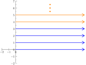
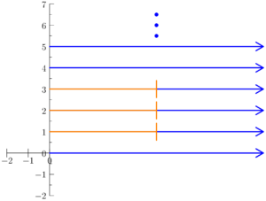
Figure 1.1.4: Here, we track the experiment described in Example 1.10 where the x-axis represents time in minutes, and the y-axis represents the number of quarters collected. In (a), we visualize what E₇ looks with orange rays. In (b), we visualize E₈ using orange segments.

Example 1.10

Consider the experiment from Example 1.5 where for an arcade machine, we record how many quarters it has collected since being turned on, and the time in minutes it takes for it to go out of service after being turned on.

Suppose we only care about outcomes where the machine has collected at least four quarters. We could describe this event as

E₇ = “The machine has collected at least 4 quarters”
E₇ = { (x, y) : x ≥ 4 }

We may only care about machines that collect between one and three quarters inclusive that are on for no longer than five minutes. In this case, we could write

E₈ = “The machine collected between 1 and 3 quarters inclusive, and is on for no longer than 5 minutes.”
E₈ = { (x, y) : 1 ≤ x ≤ 3 ∧ y ≤ 5 }

Mutually Exclusive Events

Consider the experiment of drawing a card from a well-shuffled deck again. Notice that the events

E_♣ = { (s, v) : s = ♣ }

and

E_♠ = { (s, v) : s = ♠ }

have no cards in common because no card in a standard deck has a suit that is both ♣ and ♠.

Some events may have points in common. For example the events

E_♥ = { (s, v) : s = ♥ }

and

E_J = { (s, v) : v = J }

have the card (♥, J) in common.

This kind of distinction will be important later.

Mutually Exclusive Events

Consider an experiment with sample space S.

For any two E₁ ⊆ S and E₂ ⊆ S, if

E₁ ∩ E₂ = ∅,

then E₁ and E₂ are called mutually exclusive events.