Physical Address
304 North Cardinal St.
Dorchester Center, MA 02124
Physical Address
304 North Cardinal St.
Dorchester Center, MA 02124
It can be a bit cumbersome to have to keep appealing to a multitude of theorems and axioms when trying to calculate a probability. Ideally, we shouldn’t have to keep writing what are essentially “proofs”, we just want a straight-forward calculation.
By appealing to the axioms and previous theorems a little bit more, we can formulate the process.
For some experiment with sample space S, let’s assume uniform randomness. Then for any e ∈ S, we have that

The assumption of uniform randomness gives us the following result.
Consider an experiment with sample space S under the assumption of uniform randomness.
For some event E, we have that
For any event E, we have that E ⊆ S, and as such we have that
Now, invoking Theorem 1.4.2 gives us the following:
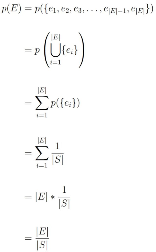
This completes the proof.
With Theorem 1.6.1, we’ve effectively turned a single probability problem into two counting problems: the first counting problem is to count the number of elements in the sample space, and the second counting problem is to count the number of elements in the event.
Once we have the two counts, we simply divide to get the probability.
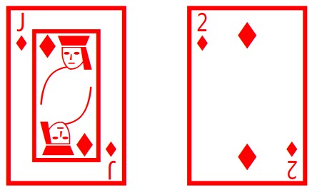
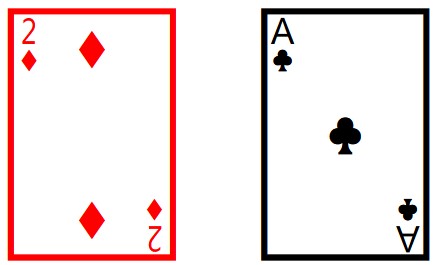
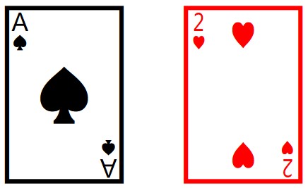
Figure 1.6.1: Here are a couple of two card draws from the experiment described in Examples 1.6.1 and 1.6.2. The card sequence in (a) does not count in either event. The sequence shown in (b) is in the event for Example 1.6.2, but not for Example 1.6.1. The sequence in (c) is in the event for both Examples 1.6.1 and 1.6.2.
Consider an experiment where we draw two cards from a well-shuffled standard deck of cards without replacement. What’s the probability that the first card is an ace, and the second card is a 2?
Since we care about what the first card is, and what the second card is, the order in which we draw cards matters. Furthermore, because there are 4 suits that a card can belong to, each ace is considered distinct from the other three aces. The same applies to the twos.
The sample space consists of all pairs of cards where no card is repeated because we draw without replacement. Thus, we have that
|S| = 52 * 51.
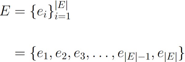
The event we care about is the event
E = { (c1, c2) : c1 is an ace ∧ c2 is a two }.
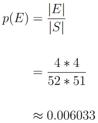
Since there are 4 aces and 4 twos, we have that
|E| = 4 * 4.
Thus, the desired probability is
Consider an experiment where we draw two cards from a well-shuffled standard deck of cards without replacement. What’s the probability that one of the cards drawn is an ace, and the other is a 2?
Here, the ace can be first and the 2 can be second, or the ace can be second while the 2 is first. Both of these occurrences are mutually exclusive, so we have that
|E| = 4*4 + 4*4.
We have the same sample space from Example 1.6.1, meaning the probability for this event is
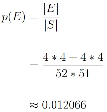
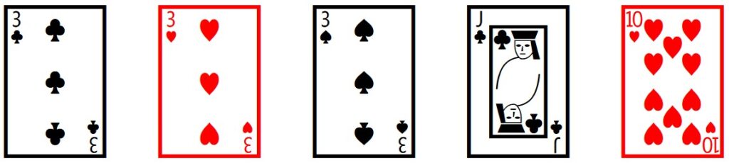
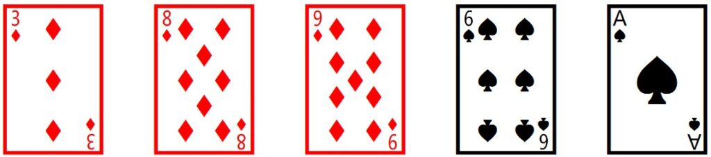

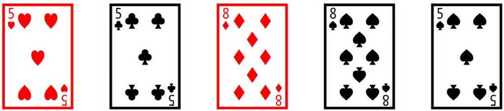
Figure 1.6.2: Here are four examples of five-card hands that can be dealt. The hand in (a) is not a full house because there is only a triple of cards with the same face value. The other two cards have different face values. (b) is not a full house because while the suits are in a triple and a pair, the face values are not. Both (c) and (d) are full houses. Since order doesn’t matter in a hand, these are actually the same full house.
Consider an experiment where we are dealt a five-card hand from a well-shuffled standard deck of cards. What is the probability that we are dealt a full house; that is, what is the probability that our hand has three cards of one face value, and two cards of a different face value?
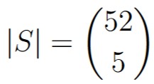
When it comes to hands, order is irrelevant. This means that our sample space for this experiment is all possible five-card hands, which is counted by the following.
We assume that no five-card hand is more likely to be dealt than any other five-card hand, and so the assumption of uniform randomness applies.
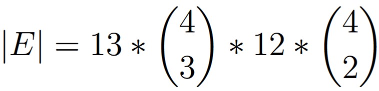
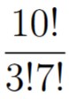
To calculate |E|, we can think in stages. First, we choose which of the 13 face values we want to represent the triple. There are 4 cards of the same face value, and we pick 3 of them without regard to order. Since there are 4 cards with the same face value, we can do this process in 13 different ways. Thus, there are

ways to choose the triple.
For the second stage, we can exclude the previous face value, leaving us with 12 face values left from which to choose. For each one of these remaining face values, we pick 2 cards from the 4 face values without regard to order, and so for the second stage, we have
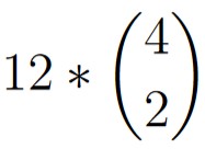
choices. Now we have a full house hand. Since we broke this down into stages, the rule of product tells us that
Thus, the probability of getting a full house is
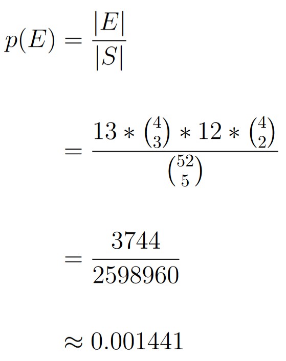
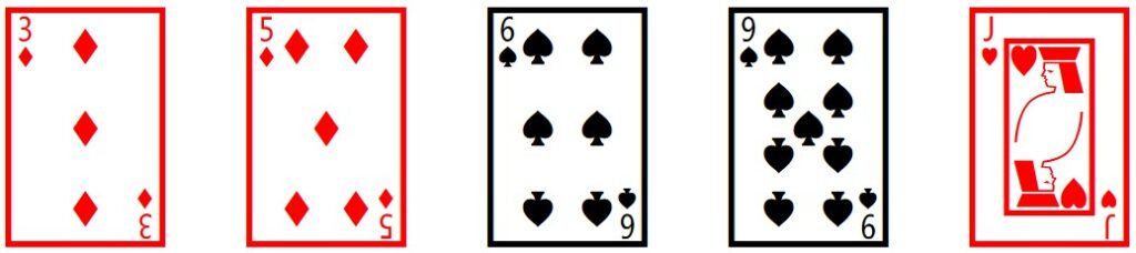
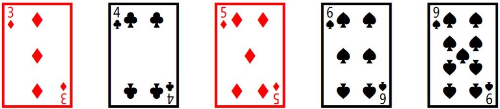
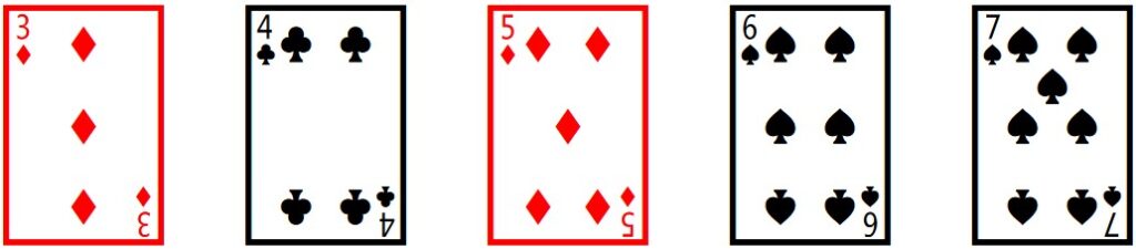

Figure 1.6.3: A straight is a hand that contains cards of sequential rank. An ace can be high or low, but it can’t make a straight from a king to a 2. So, a hand involving
Q, K, A, 2, 3
is not a straight. (a) and (b) are examples of hands that are not straights. (c) and (d) are examples of a straight, and are in fact the same straight. Note that the suits do not have to be the same.
Consider an experiment where you are dealt a five card hand. What is the probability that you are dealt a straight?
Because order is irrelevant, our sample space consists of all 5 card hands where order is not relevant. As normal, we assume that all hands are equally likely, so we have that
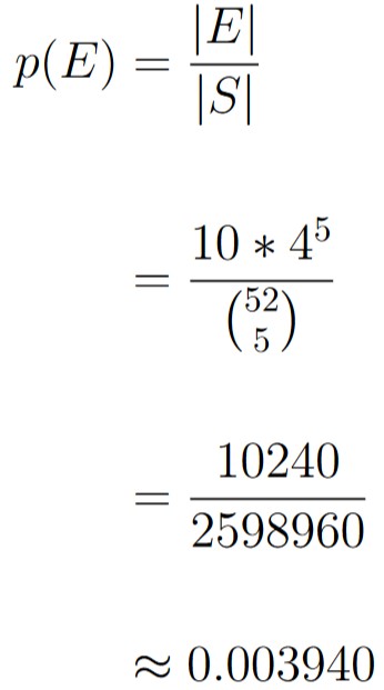
To calculate |E|, notice that there are 10 kinds of straights:
5-high, 6-high, 7-high, … king-high, ace-high.
Notice that since each card in a straight has different face value, there are 4 choices of suit for each card in the hand. As such, we have that
|E| = 10 * 45.
From this, we calculate the probability:
Consider an experiment where you shuffle a deck of cards and place it face down on the table. What is the probability that the ace of spades is closer to the top of the deck than the 2 of spades?
Notice that since we want to know the position of one card in relation to another card, order matters.
The sample space consists of all possible sequences of cards. Under the assumption of uniform randomness, we hae that
|S| = 52!.
We can calculate |E| by considering mutually exclusive cases. Suppose we number the cards where the top card is #1, and the bottom card is #52.
(♠, A) is #1 ⟹ (♠, 2) can in be in 1 of 51 spots
(♠, A) is #2 ⟹ (♠, 2) can in be in 1 of 50 spots
…
(♠, A) is #51 ⟹ (♠, 2) can in be in only be in position #52.
So, there are 51 possible locations for (♠, A), each yielding a smaller number of allowable positions for (♠, 2). However, notice that this only counts the two cards of interest. For each of these cases, there are 50! ways to arrange the other 50 cards. As such, we have that
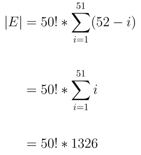
We can now calculate the probability:
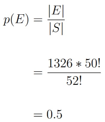
Example 1.6.5 had a remarkably simple answer for a calculation that involved very large numbers, such as 50! and 52!. We could get this result the exact same way by noticing that either (♠, A) comes before (♠, 2), or (♠, 2) comes before (♠, A). That’s only 2 possibilities, 1 of which is the possibility we want. That yields a probability of 1/2 = 0.5, same as before.
Often times, an observation about the experiment at hand can make quick work of many probability problems.
The standard approach of counting the elements of the “obvious” sample space and event is usually a good approach. However, if the answer you get looks incredibly simple, and you’ve double checked your calculations, perhaps it’s worth taking a closer look at the experiment to see if there is a more “clever” way of representing the sample space and event. This “clever” representation can often make these probability calculations much simpler, and sometimes even trivial!
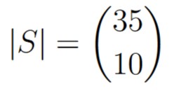
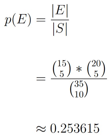
Suppose an urn contains 15 blue balls and 20 orange balls where all of the blue balls are all identical, and all orange balls are identical. Consider an experiment where you randomly draw 10 balls out of the urn without replacement. What’s the probability that you draw 5 balls of each color?
The sample space S consists of all ways to draw 10 balls out of the 15 + 20 = 35 balls from the urn. Order is not relevant here, so we have that
Because order is irrelevant, we can arbitrarily decide to count the number of ways to first select 5 blue balls from the 15 blue balls present, and then count the number of ways to select 5 orange balls from the 20 orange balls already present. The by the rule of product, we get that
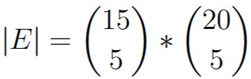
And so the probability is
In Example 1.6.6, we regarded our selections as unordered, but we could also solve this problem using ordered selections.
In order to enumerate the sample space, note that there are eleven mutually exclusive cases to consider:
| Blue Balls | Orange Balls |
|---|---|
| 0 | 10 |
| 1 | 9 |
| 2 | 8 |
| 3 | 7 |
| 4 | 6 |
| 5 | 5 |
| 6 | 4 |
| 7 | 3 |
| 8 | 2 |
| 9 | 1 |
| 10 | 0 |
For each of these cases, let nb represent the number of blue balls selected, and let no represent the number of orange balls selected. First, suppose we draw all nb blue balls first, and then draw all no orange balls, so our selection looks like the following:
⬤,⬤ , …,⬤ , ⬤, ⬤, …, ⬤.
There are
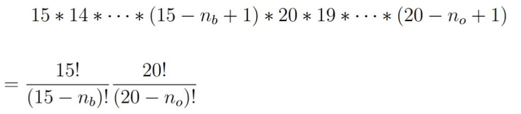
ways to draw nb blue balls and no orange balls where all blue balls come first.
For example, if nb = 3, then (since we draw 10 balls,) no =7, and our drawing would look like this:
⬤, ⬤, ⬤, ⬤, ⬤, ⬤, ⬤, ⬤, ⬤, ⬤.
And there would be
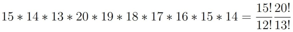
ways to select those 3 blue balls and 7 orange balls.
Now, note that the blue balls don’t have to be first; they could be dispersed around among the orange balls. For nb blue balls and no orange balls, there are
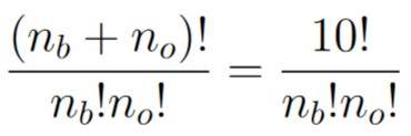
ways to arrange the drawing. So for the case where nb = 3 and no =7, there are
such arrangements.
Finally, when we account for the fact that there are eleven cases to consider, we get that our sample space has
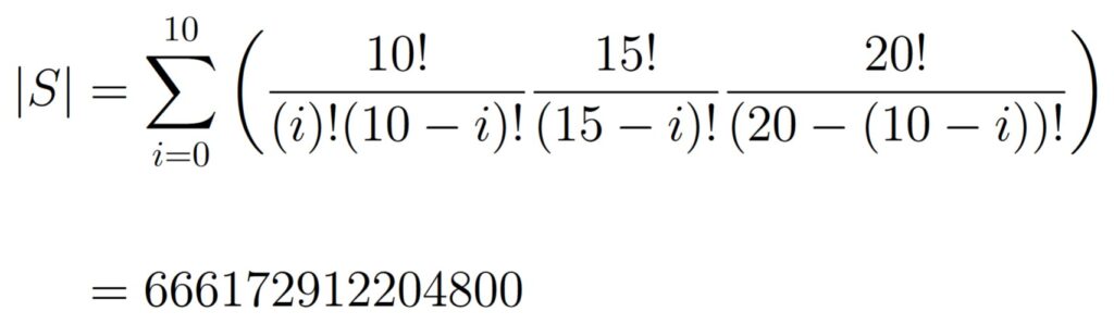
elements.
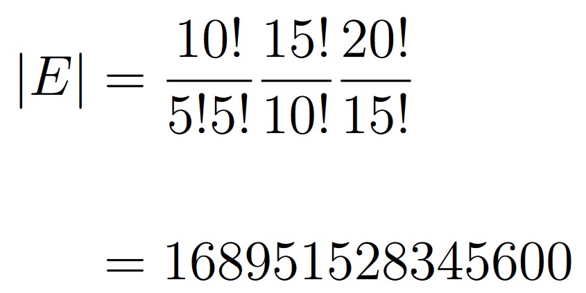
To calculate |E|, notice that we already know how to count arrangements with 5 blue balls and 5 orange balls, since that was one of the cases used to count |S|. As such, we have that
Finally, our probability is
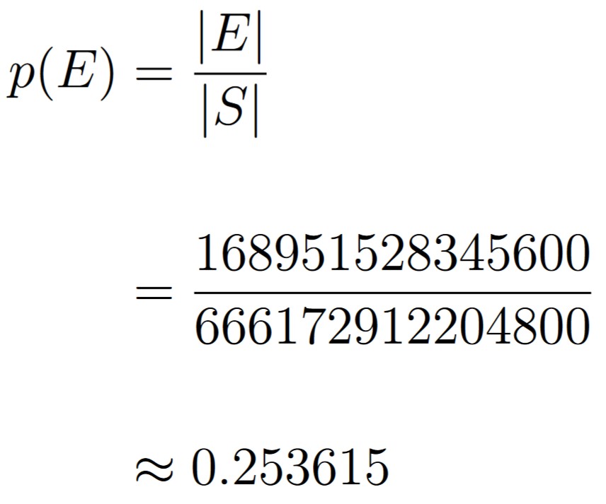
This is the same answer we got previously!
Even though we counted selections of balls from an urn in two different ways, we got the same answer. Of course, the solution presented in Example 1.6.6 seems much simpler, but there are occasions where regarding order can be beneficial. This leads to another important point worth highlighting.
Many problems of enumeration can be solved by considering how a selection would work when order is relevant, and can also be solved by disregarding order entirely. Most of the time, it one method will be easier than the other, though performing both methods can help you spot mistakes should you get two different answers.
Consider an experiment where we roll a die twice. What’s the probability that at least one roll is a six?
Our sample space S is going to consist of all ordered pairs from the Cartesian Product
S = {1, 2, 3, 4, 5, 6} ✕ {1, 2, 3, 4, 5, 6},
and so |S| = 36.
This is easy enough to list in a table:
| Roll 1 \ Roll 2 | 1 | 2 | 3 | 4 | 5 | 6 |
| 1 | (1, 1) | (1, 2) | (1, 3) | (1, 4) | (1, 5) | (1, 6) |
| 2 | (2, 1) | (2, 2) | (2, 3) | (2, 4) | (2, 5) | (2, 6) |
| 3 | (3, 1) | (3, 2) | (3, 3) | (3, 4) | (3, 5) | (3, 6) |
| 4 | (4, 1) | (4, 2) | (4, 3) | (4, 4) | (4, 5) | (4, 6) |
| 5 | (5, 1) | (5, 2) | (5, 3) | (5, 4) | (5, 5) | (5, 6) |
| 6 | (6, 1) | (6, 2) | (6, 3) | (6, 4) | (6, 5) | (6, 6) |
The event E consists of all ordered pairs with at least one 6. We can color each of those cells green.
| Roll 1 \ Roll 2 | 1 | 2 | 3 | 4 | 5 | 6 |
| 1 | (1, 1) | (1, 2) | (1, 3) | (1, 4) | (1, 5) | (1, 6) |
| 2 | (2, 1) | (2, 2) | (2, 3) | (2, 4) | (2, 5) | (2, 6) |
| 3 | (3, 1) | (3, 2) | (3, 3) | (3, 4) | (3, 5) | (3, 6) |
| 4 | (4, 1) | (4, 2) | (4, 3) | (4, 4) | (4, 5) | (4, 6) |
| 5 | (5, 1) | (5, 2) | (5, 3) | (5, 4) | (5, 5) | (5, 6) |
| 6 | (6, 1) | (6, 2) | (6, 3) | (6, 4) | (6, 5) | (6, 6) |
Here, we se that |E| = 11. Now we calculate the probability:

Consider an experiment where you roll a die four times. What’s the probability that at least one of the rolls is a six?
Similarly to Example 1.6.8, we have that
S = {1, 2, 3, 4, 5, 6} ✕ {1, 2, 3, 4, 5, 6} ✕ {1, 2, 3, 4, 5, 6} ✕ {1, 2, 3, 4, 5, 6}.
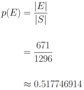
This means that |S| = 64 = 1296, which is way too many elements to conveniently list. We know that E is the event where at least one roll is a 6. However, that means that EC is the event that no roll is a 6. This means that
EC = {1, 2, 3, 4, 5} ✕ {1, 2, 3, 4, 5} ✕ {1, 2, 3, 4, 5} ✕ {1, 2, 3, 4, 5}.
As such,
|EC| = 54 = 625.
Furthermore, because E ∪ EC = S and E ∩ EC = ∅, we have that
|E| = |S| – |EC| = 1296 – 625 = 671.
Now we calculate the probability:
We can combine counting techniques with a Venn Diagram to solve probability problems as well.
The senior class at a local high school is required to have completed a course in
| A: | American History |
| B: | Biology |
| C: | Calculus |
at some point during their high school education. Let xs represent the number of students enrolled in some combination of courses during the final year; for example,
| xB | = The total number of students enrolled in Biology |
| xAC | = The total number of students enrolled in American History and Calculus |
| xABC | = The total number of students enrolled in all three courses |
Suppose we know the following information:
| xA | = 90 |
| xB | = 78 |
| xC | = 105 |
| xAB | = 34 |
| xAC | = 35 |
| xBC | = 36 |
| xABC | = 10 |
Furthermore, we also know that this senior class has 200 students. From this information, we construct the following Venn Diagram:
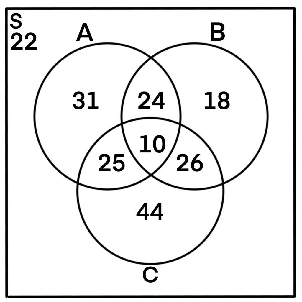
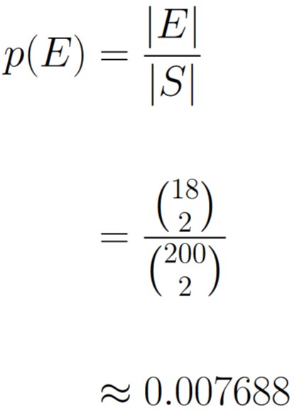
Consider an experiment where we pick two senior students at random. What’s the probability they are both only enrolled in the American History course?
The sample space S consists of every 2-student pair selected from the 200 students available. The order in which we pick the students is irrelevant, so we have that
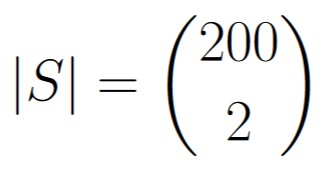
Next, the event E consists of essentially picking two students out of the 31 that are only enrolled in the American History course, and so we have that

And so, we finally have that