Geometric Probability

Based on the previous section, we know that the probability of picking individual points from an interval of real numbers is 0. This can be a problem when modeling certain phenomena such as throwing a dart at a dart board, measuring the lifetime of a light bulb, or any other situation involving a continuum of real numbers. We can’t simply count how many elements are in the sample space, nor can we count how many elements are in the desired event. This is because the real numbers are uncountably infinite.

Picking Points from an Interval

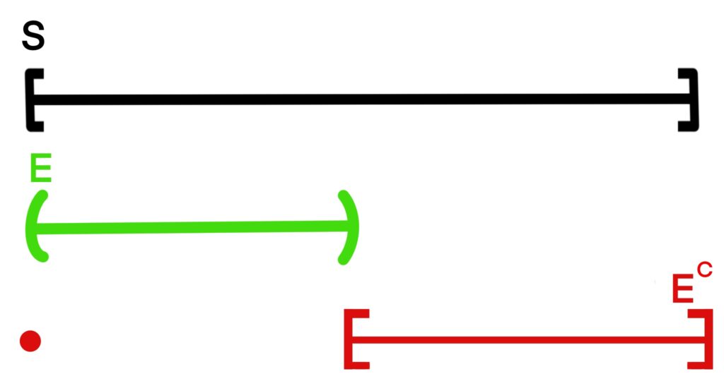
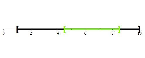
Figure 1.9.1.: When randomly picking a point from [0, 1], we can ask about what kinds of intervals the point resides. Here, the green sub component of [0, 1] represents the interval (0, 0.5). The red sub component represents everything else in [0, 1] that is not in E.

Suppose we’re working with the interval [0, 1]. As stated before, the probability of picking a specific point from this interval is 0. Instead of trying to pick specific points from the interval, let’s reframe the problem in the following way: what’s the probability that a randomly selected point falls in the interval (0, 0.5)? Let p( (0, 0.5) ) denote the probability that the point is in the interval (0, 0.5).

Let p(0) denote the probability that the randomly selected point is 0, and let p(0.5) be defined analogously. Because p(0) = p(0.5) = 0, including the endpoints of interval (0, 0.5) will not affect the probability of a randomly selected point falling within that interval. That is to say,

p( (0, 0.5) ) = p( [0, 0.5) ) = p( (0, 0.5] ) = p( [0, 0.5] ).

Using the terminology of sample spaces and events, we would say that

S = [0, 1], E = (0, 0.5).

By this logic, we would define the complementary event E^C as

E^C = {0} ∪ [0.5, 1].

Appealing to the Axioms

Because

p( (0, 0.5) ) = p( [0, 0.5) ) = p( (0, 0.5] ) = p( [0, 0.5] ),

and because

p( (0.5,1 ) ) = p( [0.5, 1) ) = p( (0.5, 1] ) = p( [0.5, 1] ),

we can just redefine E and E^C as follows:

E = [0, 0.5), E^C = [0.5, 1],

giving us that

E ∪ E^C = S.

Now we can appeal to the axioms of probability, as well as any previous theorems we’ve proven. Recall that by Axiom 2,

p(S) = 1.

By Theorem 1.4.2, we also have that

p(E) + p(E^C ) = p(S).

Notice that the length of interval [0, 0.5) = 0.5, and the length of [0.5, 1] is also 0.5. Because [0, 0.5) and [0.5, 1] are mutually exclusive intervals of equal length, we assume uniform randomness, giving us that

p(E) = p(E^C).

From this, we get the following:

p(E) + p(E^C ) = p(S)	⟹	p(E) + p(E^C ) = 1
	⟹	p(E) + p(E) = 1
	⟹	2p(E) = 1
	⟹	p(E) = 0.5

So, the probability that a randomly chosen point from [0, 1] will be in the interval [0, 0.5) is 0.5. Just to reiterate, this also tells us that

p( (0, 0.5) ) = p( [0, 0.5) ) = p( (0, 0.5] ) = p( [0, 0.5] ) = 0.5.

A More Intuitive Approach

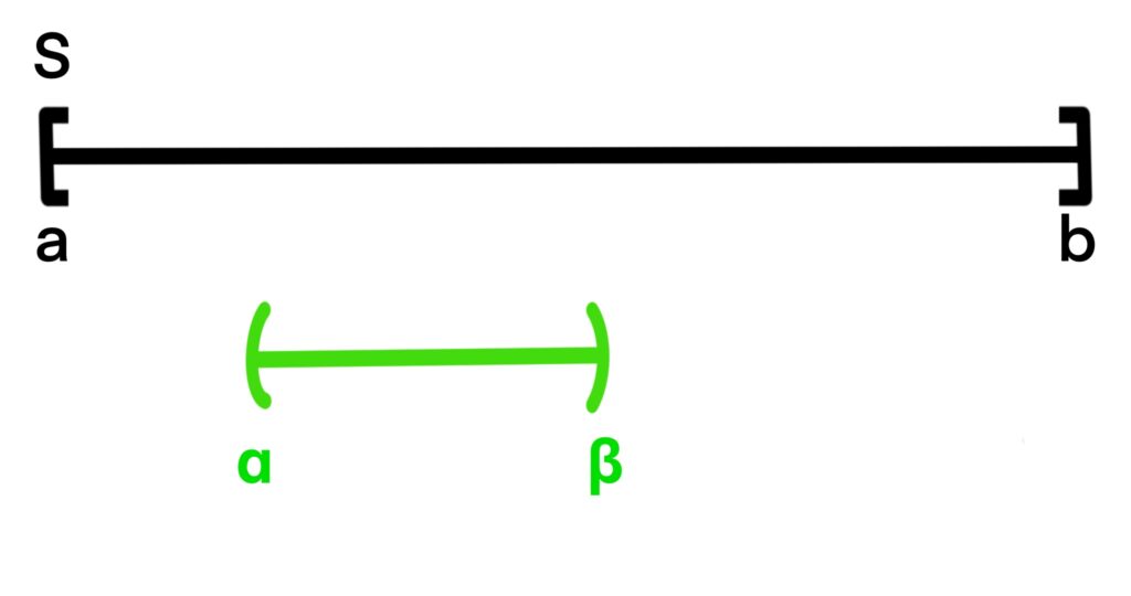
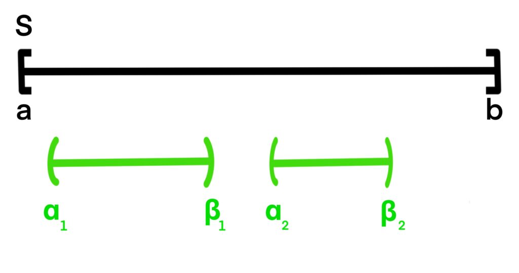
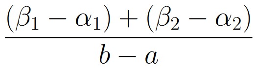
Figure 1.9.2: Geometric probability is calculated by dividing the length of the “desired region” by the length of the total region. In (a), this means that the probability a randomly selected point appears in (α, β) is

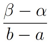In (b), with the desired region being split across two intervals, we simply add their lengths, so the probability a randomly chosen point appears in either green region is

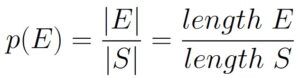
Instead of going through the process of appealing to the axioms, and assuming uniform randomness, we can instead extend Theorem 1.6.1 by denoting the length of the interval represented by E as |E|. Likewise, we use |S| to refer to the length of the the interval associated with S.

Example 1.9.1

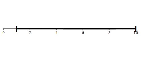
You and a friend are playing a game where you both guess any real number between 1 and 10 inclusive. If your number is within 2 of your friend’s number you win.

For example, if you pick the number 5, then if your friend’s number is in the interval

[5 – 2, 5 + 2] = [3, 7],

then you win. Likewise, if you pick 3.5, then you win if your friend picks a number in the interval

[3.5 – 2, 3.5 + 2] = [1.5, 5.5].

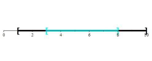
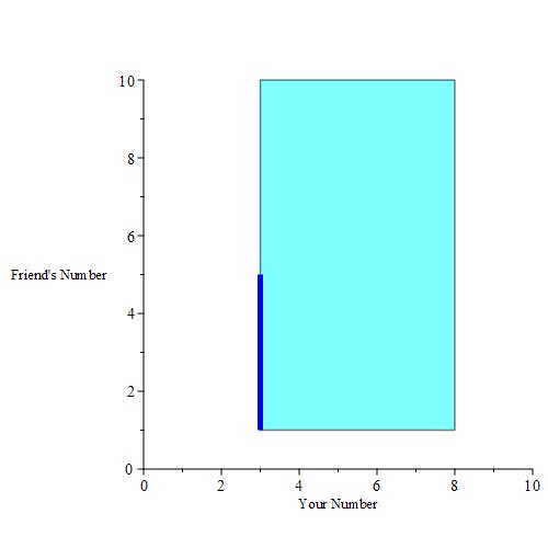
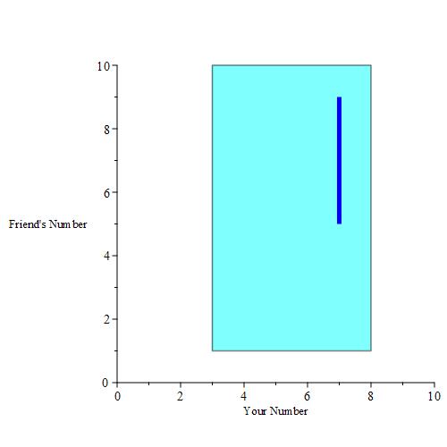
Of course, you don’t want to pick any number in the interval [1, 3), and you don’t want to pick a number from (8, 10] because you won’t be able to take full advantage of the length 2 buffer region around those numbers. Essentially, this means that you will only pick numbers from the interval [3, 8] to maximize your chance of winning. This portion of the line is represented by the blue region of the below image.

What is the probability that you win?

We know that

|S| = 10 – 1 = 9.

For any number x you pick, you win if your friend’s number is in [x – 2, x + 2], which has a length of

|E| = (x + 2) – (x – 2) = 4.

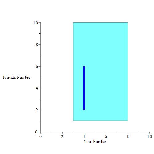
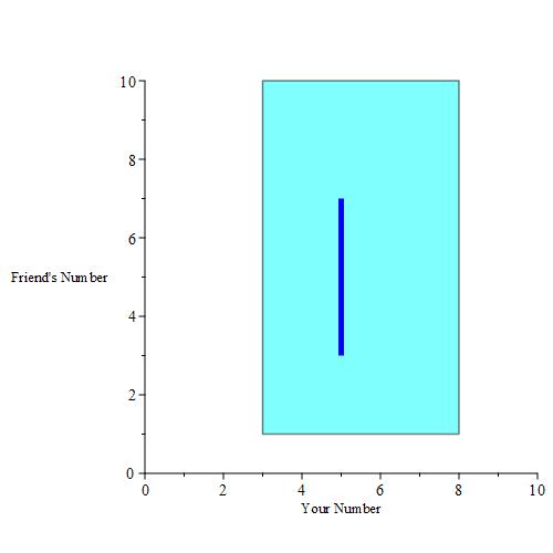
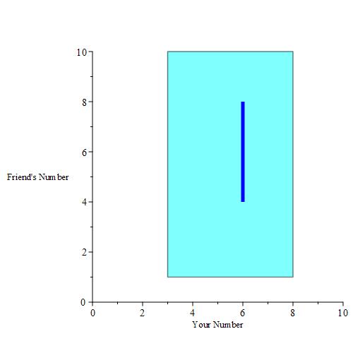
So, if you were to pick x = 3, or x = 6.5, you would win if your friend picked any number in the following green regions:

Since the length of the desired region is always 4, we have that

Based on this more intuitive approach, we make the following definition:

Randomly Selected Point from an Interval

A point is said to be a randomly selected point from an interval (a, b) if any two sub-intervals

(α₁, β₁), (α₂, β₂)

with the same length are both equally likely to contain the randomly selected point.

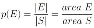
The probability that the randomly selected point is contained within the sub-interval (α, β) of interval (a, b) is defined to be

Probability in Two Dimensions

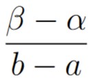
Figure 1.9.3: In two dimensions, we specify areas. In (a), we define the engrossing region S as the pictured blue square. S has a width and height of

x₂ – x₁, y₂ – y₁

respectively. In (b), we define a green subregion E of the square in which we want a randomly selected point to reside. The green square E has a width and height of

α₂ – α₁, β₂ – β₁

respectively.

When we deal with picking points on a real number line, we have to specify regions of interest instead of specific points. For the exact same reasons, when we deal with the plane, we also have to specify regions of interest. Whereas in one-dimension we only specify one interval, in two dimensions, we must specify two intervals.

More specifically, if we are interested in randomly picking points (x, y) in the plane, we need to specify an interval of interest for the x-coordinate, and an interval of interest for the y-coordinate. This naturally leads us to calculate probabilities using areas instead of lengths.

Example 1.9.2

Consider the game described from Example 1.9.1 above. We can use areas to calculate the probability of winning. First, we should get a handle of the geometric region with which we’re dealing.

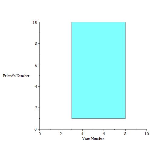
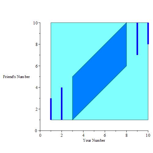
You want to maximize your chances of winning, so you only want to pick a number in the interval [3, 8]. Your friend can pick any number in the interval [1, 10]. Let your number be x, and let your friend’s number be y. We can now plot the region of interest as a blue rectangle.

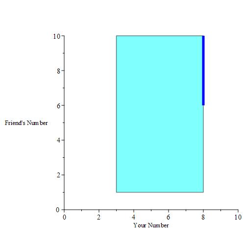
If you pick a number, then you are essentially given a buffer. We can plot those buffers when you pick 3, 4, 5, 6, 7and 8 for example. This is the result when those buffer regions are colored a dark blue color.

Of course, we could pick any real number in [3, 8], including 3.14, 5.6672, e * 2, and so on. A plot of all of these points yields a solid parallelogram as depicted below.

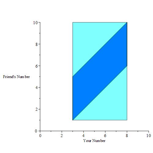
These are shapes for which we can easily calculate the area. The region S, depicted by the light blue/cyan rectangle has an area of

|S| = (10 – 1) * (8 – 3) = 9 * 5 = 45.

The dark blue parallelogram has a base length of 4 (the length of the vertical cross sections) and a width of (8 – 3) = 5. This tells us that

|E| = 4 * 5 = 20.

And so, we calculate the probability to be

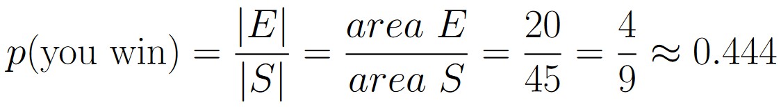
This is the exact same answer we got in Example 1.9.1. Once again, we’ve used two different methods to solve a problem, and arrived at the exact same answer each time.

Example 1.9.3

Consider the game presented in Example 1.9.1 again. Suppose you like to live a little bit dangerously and are O.K. with picking numbers from the entire interval [1, 10]. If you randomly select a point from that interval, what’s the probability that you win now?

This time, you can pick the number 1, meaning you win if your friend picks a number in the interval [1, 3]. If you pick 2, then you win if your friend picks any real number in the interval [1, 4]. On the other end of the spectrum, if you pick 10, you win if your friend picks a number in the interval [8, 10]. If you pick 9, then you win if your friend picks a number in the interval [7, 10].

Just as before, there is a continuum of values you can pick in the interval [1, 3] as well as [8, 10]. If we color in all successful points a dark blue color, we get the following figure.

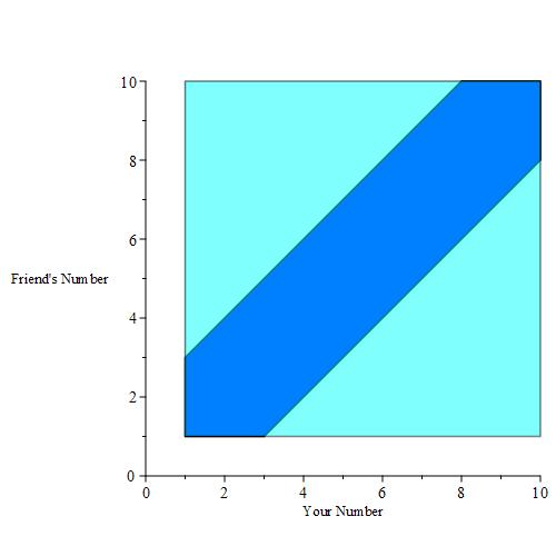
To calculate the probability of winning, we need to calculate |S| and |E|. We can easily calculate |S|:

|S| = (10 – 1) * (10 – 1) = 9 * 9 = 81.

To calculate |E|, one thing we can do is calculate the area of the two light blue triangles, and subtract from the area of the overall square (which has area |S| = 81). The area of the bottom-right light blue triangle is

0.5 * (10 – 3) * (8 – 1) = 0.5 * 7 * 7 = 24.5.

The area of the upper-left light blue triangle is

0.5 * (8 – 1) * (10 – 3) = 0.5 * 7 * 7 = 24.5.

Now, we know that the area of the dark blue shape is

|E| = 81 – 24.5 – 24.5 = 32.

Finally, we calculate the probability that you win:

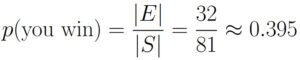
This time, the probability that you win is roughly 0.395, which is slightly less than your probability of winning if you restrict your number to the interval [3, 8]. In summary, you should stick with your previous strategy.

Probability in Three Dimensions

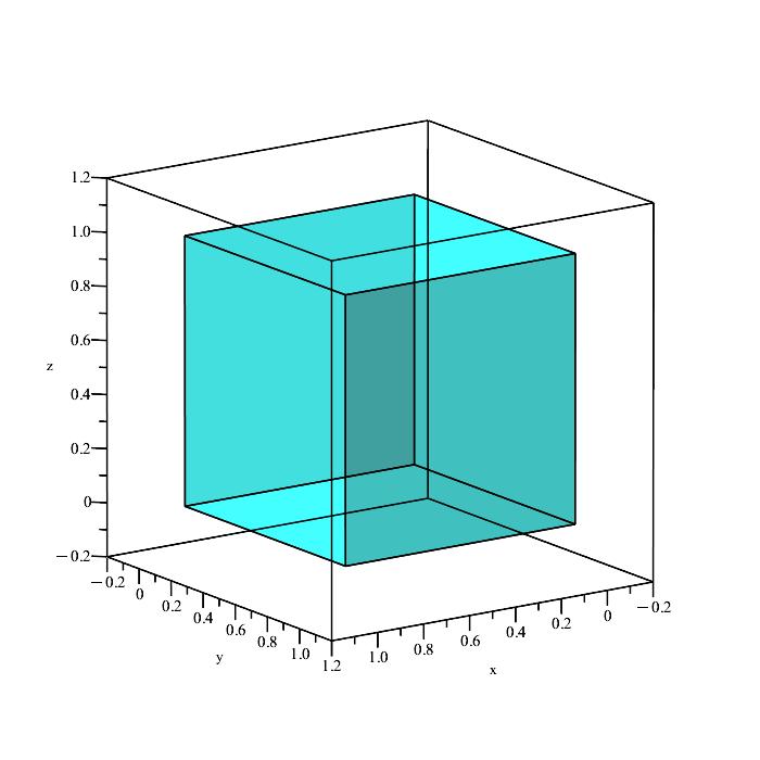
Extending from two dimensions to three dimensions involves specifying possible values for a third variable, just like what we do when going from one dimension to two dimensions. Specifying bounds for three variables is analogous to specifying volumes in three dimensional space.

Example 1.9.4

Suppose you pick thee points x, y, and z at random from the interval [0, 1]. What is the probability that

x ≤ y ≤ z?

For any probability problem, we can start by getting a grip of what the sample space is. In this case, we have three points satisfying the following restrictions:

x ∈ [0, 1], y ∈ [0, 1], z ∈ [0, 1].

This is just a unit cube in three dimensional space. We can look all around the cube to get a sense of how big the cube is within space. The unit cube has a volume of 1, and so |S| = 1.

Now we need to get a sense of what our event looks like in 3D space. We essentially have three conditions to satisfy:

x ≤ y, y ≤ z, x ≤ z.

We can quickly plot the boundaries of these conditions to see what is happening.

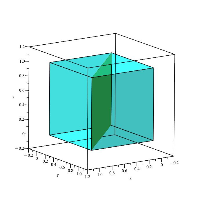
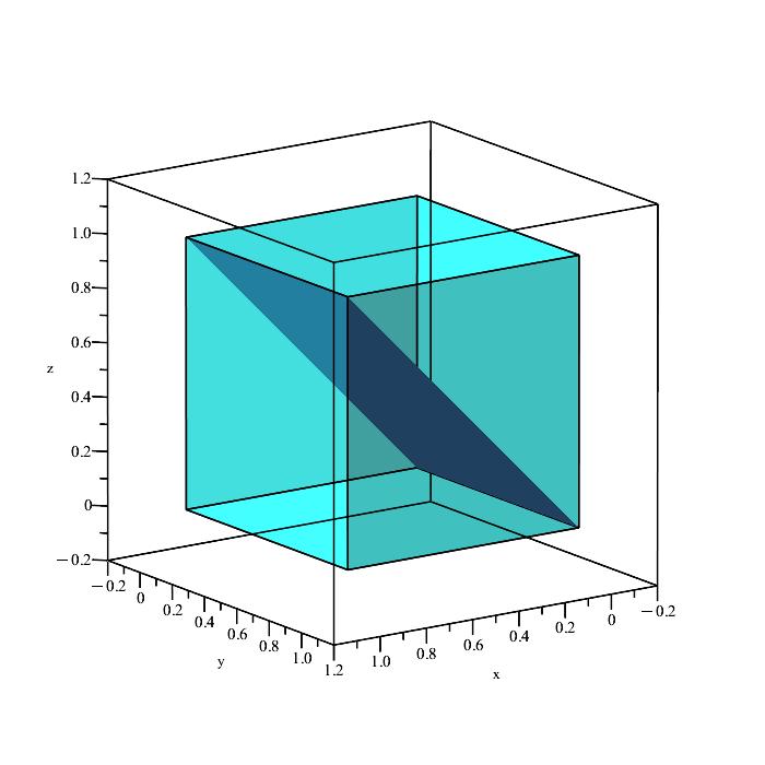
Remember that the region in space containing all points satisfying the inequalities

x ≤ y, y ≤ z, x ≤ z,

is a solid volume, not a plane (the above planes are only showing the boundaries because they depict the equalities x = y, y = z, and x = z.)

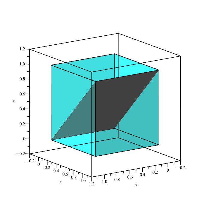
We know the boundaries, but what does the region of space look like? We can start by examining the extremal points of the cube:

(0, 0, 0), (0, 0, 1), (0, 1, 0), (0, 1, 1), (1, 0, 0), (1, 0, 1), (1, 1, 0), (1, 1, 1).

Notice that only 4 of these extremal points satisfy the desired inequalities. Below, we color the desired extremal points green, and the undesired extremal points red:

(0, 0, 0), (0, 0, 1), (0, 1, 0), (0, 1, 1), (1, 0, 0), (1, 0, 1), (1, 1, 0), (1, 1, 1).

Those four green points represent the extremities of the desired region in space we want. Every point boiunded by those extremities is also included. The solid volume containing all the points we want is depicted below.

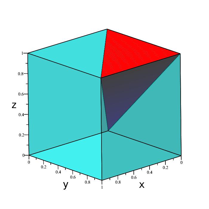
The region is a triangular pyramid, and as such has volume

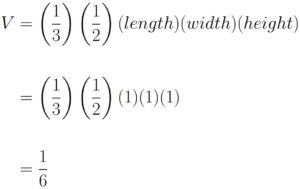
Since |E| = V, we can now calculate the probability:

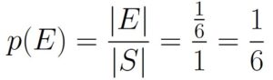
As a reminder, we can sometimes avoid going through a bunch of calculations to get the final answer. We can do this by thinking about how to count or measure the size of the event in different ways. The next example is another demonstration of this fact.

Example 1.9.5

Suppose you pick thee points x, y, and z at random from the interval [0, 1]. What is the probability that

x ≤ y ≤ z?

Suppose we just pick a random point from within the unit cube (a, b, c). There are 3! = 6 possible ways to order a, b, and c from least to greatest:

a ≤ b ≤ c
a ≤ c ≤ b
b ≤ a ≤ c
b ≤ c ≤ a
c ≤ a ≤ b
c ≤ b ≤ a.

The only ordering satisfying the requirement is a ≤ b ≤ c. As such the probability is

This is the exact same answer we got in Example 1.9.4.