Physical Address
304 North Cardinal St.
Dorchester Center, MA 02124
Physical Address
304 North Cardinal St.
Dorchester Center, MA 02124
Before Kolmogorov formulated the modern axiomatic approach to probability theory, there was the relative frequency interpretation of probability. To formulate the definition of probability using this interpretation, suppose Ω represents some event of an experiment. We perform n trials of the experiment, and we define n(Ω) as the number of times event Ω occurred during those n trials. We could then define the probability of Ω occurring, denoted p(Ω), as
Obviously, we would never be able to conduct an experiment infinitely many times. Furthermore, we can’t necessarily expect the limit to even exist. If it does exist (perhaps existence is assumed axiomatically,) then there is no reason to believe that the limit is always the same value when different sets of experiments are conducted.
Nevertheless, we can still make use of this definition. Even if we can’t perform an infinite number of experiments, with automation, we could perform many experiments. Indeed, we can develop programs to perform large numbers of experiments.
The main tool used to perform these experiments will be a random number generator, but we have to be able to model experiments using random numbers. For example, if our experiment is to flip a coin, we can use 0 to represent tails and a 1 to represent heads. We could generate integers from 1 to 6 inclusively to simulate a dice roll. If we want to pick points on a line or in a plane, we could generate real numbers from 0 to 1 to form points. The idea is that, once we have a model for how we represent outcomes in an experiment, we can automate experiments in code.
Random number generation is relatively easy with a tool like Maple. In addition to providing facilities for producing random numbers, Maple also allows us to easily visualize the outcomes of experiments (Maple has been used extensively to produce most of the images used in this book thus far.)
Modeling a coin flip using numbers is pretty straightforward. We simply use a 0 to represent an outcome of “tails”, and we use a 1 to represent an outcome of “heads.”
With that model in place, now all we have to do is automate generating 0s and 1s. We’ll simulate a fair coin, so we want these 0s and 1s to be generated uniformly each time. We’ll collect all of the results in a list so that way we can calculate cumulative frequencies for flipping heads.
After we calculate the cumulative frequencies, we’ll visualize the results with a line chart. The line chart will show us where the ratios of flipping heads and flipping tails tend towards.
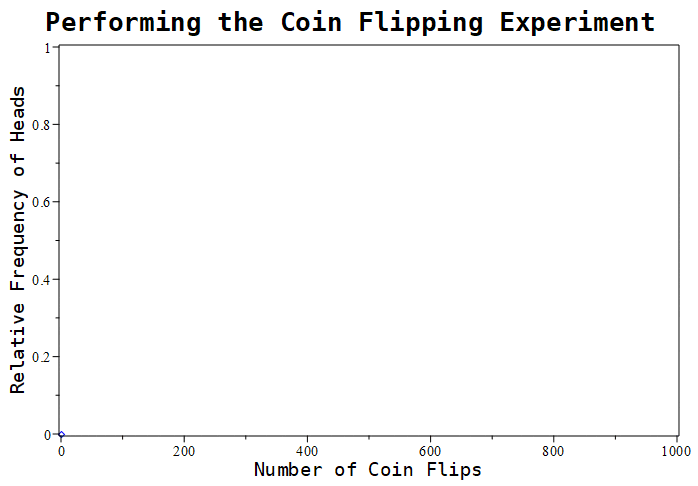
Figure 1.11.1: As we flip the coin more and more, the ratio of heads to tails tends to stabilize around 0.5, which is what the theoretical probability of landing heads after flipping a fair coin would be.
restart:
with(Statistics):
with(RandomTools):
with(ListTools):
with(plots):
with(plottools):
Performing the Experiment
number_flips := 1000:
randomize():
sample_flips := Generate(list(nonnegint(range = 1), number_flips)):
Calculating the Cumulative Frequency
data_indices := [seq(1..number_flips)]:
sample_cumulative_sums := PartialSums(sample_flips):
sample_cumulative_frequencies := sample_cumulative_sums /~ data_indices :
Displaying the Results
plot_1 := LineChart(
sample_cumulative_frequencies,
view = [0..number_flips, 0..1],
color = “Blue”,
labels = [“Number of Coin Flips”, “Relative Frequency”],
labelfont = [“Courier”, “roman”, 15]
):
plot_2 := line(
[0, 0.5], [number_flips, 0.5],
color = “Orange”,
thickness = 3
):
display(
[plot_1, plot_2],
view = [0..number_flips, 0..1],
title = “Comparing the elative Frequency to the Theoretical Probability”,
titlefont = [“Courier”, “bold”, 20],
legend = [“Relative Frequency”, “Theoretical Probability”],
legendstyle = [font = [“Courier”, “roman”, 20]]
)
Animating the Line Chart
F_1 := proc(n)
LineChart(
sample_cumulative_frequencies[1..n],
color=”Blue”
);
end proc:
animate(
F_1, [n], n = [seq(1..number_flips)],
view = [0..number_flips, 0..1],
paraminfo = false,
title = “Performing the Coin FLipping Experiment”,
titlefont = [“Courier”, “Bold”, 20],
labels = [“Number of Coin Flips”, “Relative Frequency of Heads”],
labelfont = [“Courier”, “roman”, 15]
)
Notice that in the above Maple document, we set the number of samples to 1000. That is, we are going to generate 1000 numbers. We can specify any number of flips we want to perform and generate the appropriate charts. Below, we’ll display the charts generated for when we specify 10, 100, and 1000 coin flips respectively. This is done to show what generally happens as the number of samples you take gets larger and larger.
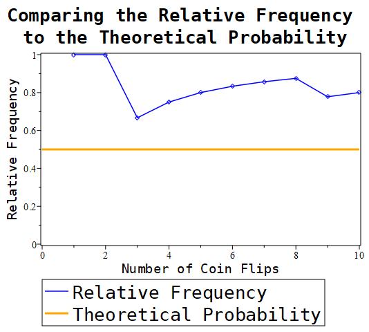

Figure 1.11.2: As can be seen, the more samples that are taken, the more and more the ratio seems to be approaching the value 0.5.
For this experiment, each sample requires us to roll two dice. We then add those dice up to get the sum of those dice. After rolling multiple times, we’ll have the data, and we can display them in a bar chart.
This time, we can generate two lists of random integers between 1 and 6 inclusive. We then pairwise add together both lists to get the desired sums. The Maple code for this simulation is presented below.
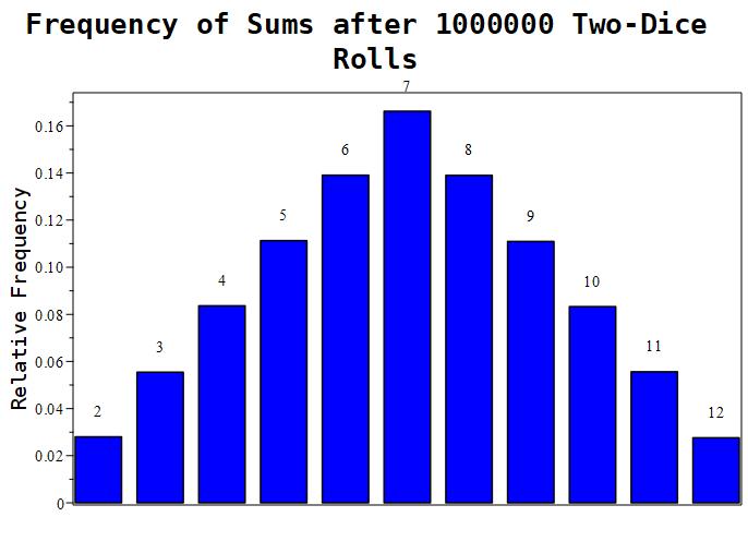
Figure 1.11.3: Here are the frequencies of sums we get after simulating 1000000 pairs of dice rolls. These results are congruent with our earlier calculations where we calculated the probability of rolling a sum of 7 to be roughly 0.16667.
restart:
with(Statistics):
with(RandomTools):
with(ListTools):
with(plots):
with(plottools):
Performing the Experiment
number_rolls := 1000000:
sides := 6:
randomize():
sample_rolls_1 := Generate(list(posint(range = sides), number_rolls)):
sample_rolls_2 := Generate(list(posint(range = sides), number_rolls)):
sample_sums := sample_rolls_1 +~ sample_rolls_2:
Generate The Bar Chart
sample_data := Tally(sample_sums, output=table):
sample_frequencies := [entries(sample_data, ‘nolist’)] /~ number_rolls:
bar_labels := [seq(2..12)]:
ColumnGraph(
sample_frequencies,
datasetlabels = bar_labels,
color = “Blue”,
title = cat(“Frequency of Sums after “, number_rolls, ” Two-Dice Rolls”),
titlefont = [“Courier”, “bold”, 20],
labels = [“”, “Relative Frequency”],
labeldirections = [“horizontal”, “vertical”],
labelfont = [“Courier”, “roman”, 15]
)
With this program, we can quickly change how many samples we take. For example, we can compare the results we get by taking 10, 100, and 1000 samples, displayed immediately below.
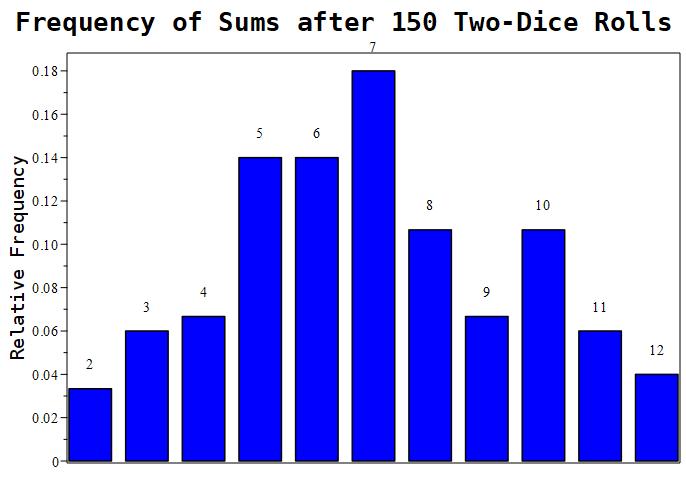
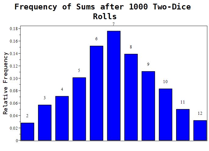
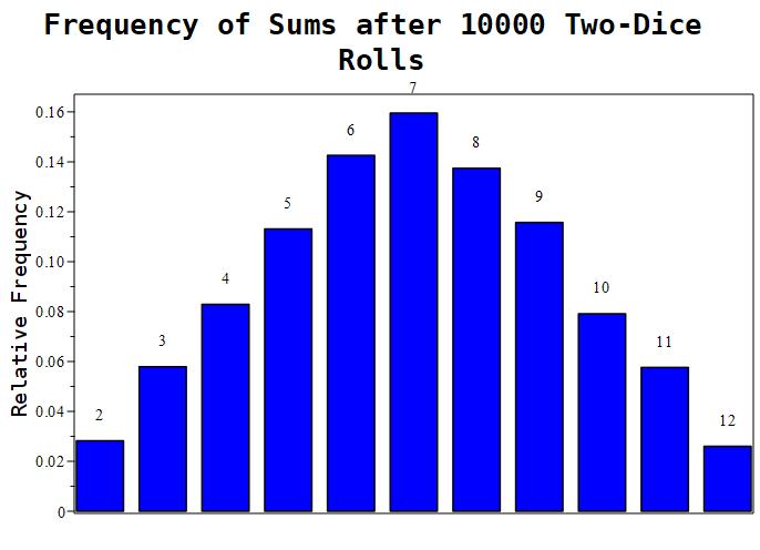
Figure 1.11.4: Here are the results of 3 experiments. The leftmost image depicts an experiment with 10 samples. The middle picture depicts an experiment with 100 samples. The rightmost image depicts an experiment with 1000 samples. As more and more samples are taken, we see that numbers closer to 7 are more likely to be rolled.
The above script can easily be extended to estimate the probability of rolling a 7. Repeating this experiment with ever-larger sample numbers, we get the following data.
| Number of Samples | 10 | 100 | 1000 | 10000 | 100000 | 1000000 |
|---|---|---|---|---|---|---|
| Number of times the sum was 7 | 3 | 17 | 163 | 1629 | 16471 | 166149 |
| Ratio of samples where the sum is 7 | 0.3 | 0.17 | 0.163 | 0.1629 | 0.16471 | 0.166149 |
Using probability theory, we calculate the probability of two dice summing to be 7 to be 1/6 ≈ 0.1667. We notice that the experiments with larger samples tend to yield estimates close to 1/6.
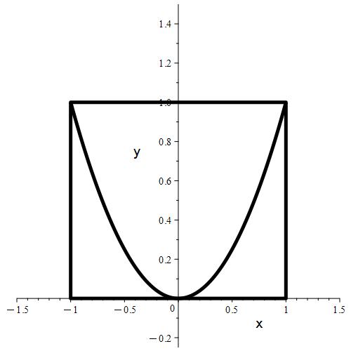
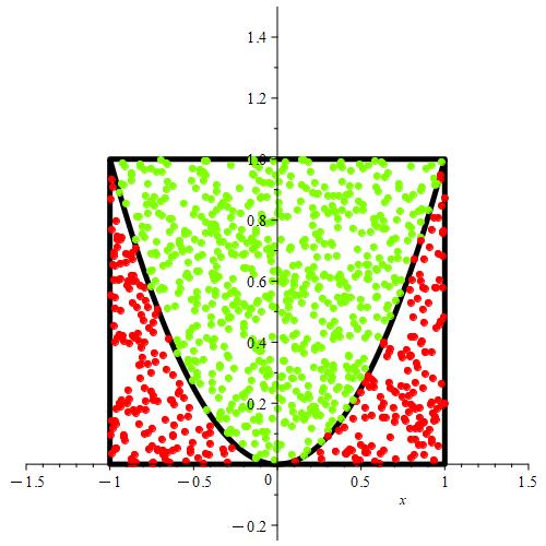
Figure 1.11.5: In (a), we show a graphical representation of the region from which points will be randomly selected, represented by the rectangle. The parabola represents the equation
y = x2,
which represents the boundary of points that either meet or reject the imposed condition. Basically, we’re trying to estimate the probability that a randomly selected point from the rectangle will be above the parabola. In (b), we show a selection of 1000 points. Notice that any points satisfying the condition are colored green, while any points not satisfying the condition are colored red.
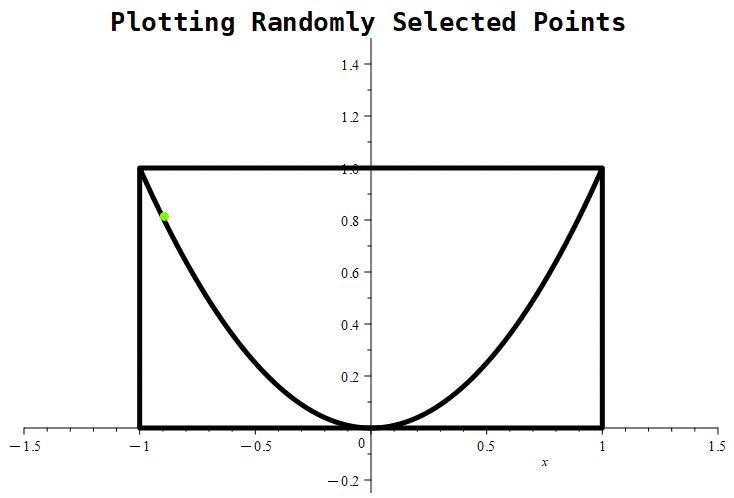
Figure 1.11.6: Here, we see the simulation in progress where we place 1000 randomly chosen points.
In this simulation, we’re going to estimate the probability that any randomly chosen point (x, y) with
x ∈ [-1, 1] and y ∈ [0, 1]
satisfies the condition that
y ≥ x2.
We begin by generating a list of x values, and a separate list of y values. The first list will generate real numbers from the interval [-1, 1]. The second will generate real numbers from the interval [0, 1].
After generating lots of sample points, we count how many of those points satisfy the condition. We then divide that number by the total number of points generated. This will yield our estimate for the probability.
We can track the cumulative frequency to see where, with more and more generated points, the probability estimate tends towards. We can most easily see this with a line chart.
restart:
with(Statistics):
with(RandomTools):
with(plots):
with(plottools):
Defining the Function
boundary := x → x2:
Generating the Sample Data
lower_x := -1.0:
upper_x := 1.0:
lower_y := 0:
upper_y := 1.0:
number_samples := 1000:
randomize():
sample_x := Generate(list(float(range=lower_x..upper_x, method=uniform), number_samples)):
sample_y := Generate(list(float(range=lower_y..upper_y, method=uniform), number_samples)):
sample_data := [sample_x, sample_y]:
Coloring the Points for Visual Clarity
sample_colors := []:
for i from 1 to number_samples do
if sample_x[i]2 ≤ sample_y[i] then
sample_colors := [op(sample_colors), “Chartreuse”]
else
sample_colors := [op(sample_colors), “Red”]
end if
end do
Counting Points Satisfying the Condition
sample_checks := []:
for i from 1 to number_samples do
if sample_x[i]2 ≤ sample_y[i] then
sample_checks := [op(sample_checks), 1]
else
sample_checks := [op(sample_checks), 0]
end if
end do
Calculating The Cumulative Frequency
data_indices := [seq(1..number_samples)]:
cumulative_sums := CumulativeSum(sample_checks):
cumulative_frequencies := cumulative_sums /~ data_indices:
Displaying the Boundaries
box_plot := rectangle([lower_x, lower_y], [upper_x, upper_y], color = “Black”, style = line, thickness = 5):
boundary_plot := plot(boundary(x), x = lower_x..upper_x, color = “Black”, thickness = 5):
Constructing the Scatter Plot
F_1 := proc(n)
display(
[
box_plot, boundary_plot,
pointplot([sample_x[1..n], sample_y[1..n]], color = sample_colors[1..n], symbol = solidcircle)
],
view = [-1.5..1.5, -0.25..1.5],
title = “Plotting Randomly Selected Points”,
titlefont = [“Courier”, “bold”, 20]
)
end proc:
Constructing the Line Chart
F_2 := proc(n)
LineChart(
cumulative_frequencies[1..n],
view = [0..number_samples, 0..1],
title = cat(“Cumulative Frequency = “, evalf5(cumulative_frequencies[n])),
titlefont = [“Courier”, “bold”, 20]
)
end proc:
Side by Side Plots
my_plots := [seq(display(Array([F_1(n), F_2(n)])), n = 1..number_samples)]:
my_display :=display(my_plots, insequence = true)
We’ll show the results of 3 different simulations: the first one will show the results of randomly selecting 10 points, the second will show a sample of 100 randomly selected points, and the third will show a sample of 1000 randomly selected points.
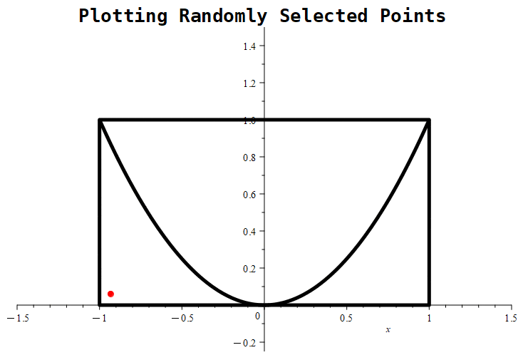
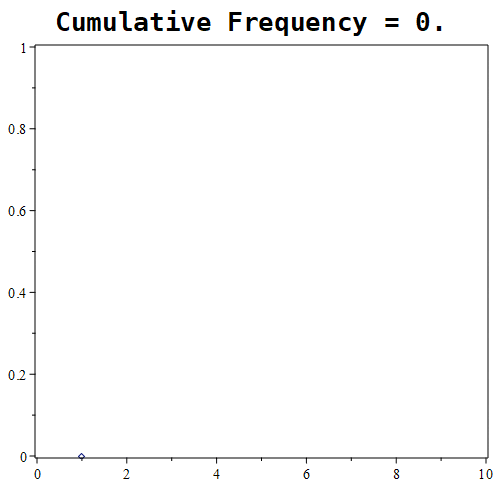

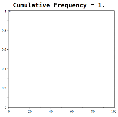
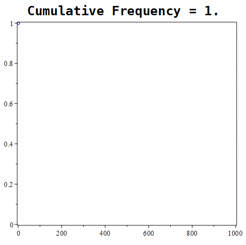
Figure 1.11.7: Here are the results of placing 10, 100, and 1000 randomly generated points. Notice that the probability roughly approaches a value of around 0.5 in the first graph, whereas in the middle graph, the estimate being tracked is approaching a value of nearly 0.61. With 1000 points, the estimate is nearly 0.667.
Of course, 10 points will likely not be a good number of samples. Statistical theory is the bedrock of any good experimental design. While there are statistical tools to help us decide on a number of samples to take, a good rule of thumb is that more is better, so we’ll just arbitrarily increase the number of samples to 1000.
Looking at the experiment where we randomly select 1000 points, the relative frequency tends towards roughly 0.6676. How good of an estimate is that?
As discussed in the section on geometric probability, we can calculate the theoretical probability by dividing the area of the desired region by the area of the total region from which points are selected. If we let E be the event where the point we randomly select is in the desired region, we have the following result.
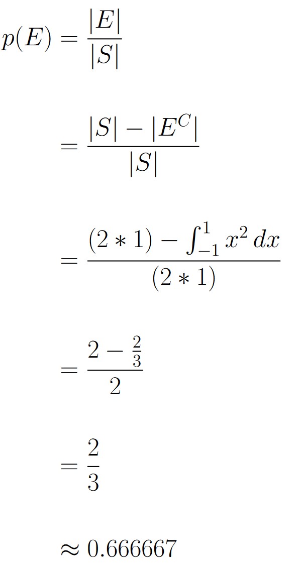
So, it appears our estimate is very close to the theoretical probability we just calculated.