Conditional Probability

In the previous chapter, we’ve developed a lot of probability theory by defining simple terms and building up logic from the axioms. Here, we’ll continue to build up the theory.

The primary way we’ll do this is by taking another look at the sample spaces of various experiments. In some cases, we may not be interested in examining events from the entire sample space; instead, we may be more interested in events that have imposed conditions. Put another way, we may only be interested in events coming from some subset of the sample space.

Some Motivating Example Problems

Card 1

🃜 🃜

Card 2

🃜 🃜

Figure 2.1.1: The game involves two cards. Shown above is a visual representation.

Example 2.1.1

Suppose a street hustler invites you to play a simple card game where she has two cards. One card is black on both sides. The other card has a red side and a black side. She says you win if the card she deals has the red face showing.

At first, she shuffles the cards and chooses one at random (she is not being sneaky here, so the card dealing is done fairly and perfectly randomly.) What’s the probability that you win?

In this situation, there are 4 possible faces that could show, only 1 of which has the red face, so the probability that you win is 1 / 4 = 0.25. This means you lose with probability 3 / 4 = 0.75.

Example 2.1.2

Because the probability that you lose the game described in Example 2.1.1 is so high, the street hustler proposes the following change: she will still deal a card at random, and if it shows red, you win $1. However, if the card has a black face showing, you are allowed to flip the card over. If you decide not to flip the card, you walk away without losing or gaining any money. If you flip the card and it shows black, you lose $1, but if it shows red you win $1.

Again, she fairly deals out a card at random, and it is showing a black face. What is the probability that the other side is red?

We can model this game as a two stage process: the first stage involves picking one out of the four possible faces to show. The second stage involves flipping the card over to reveal the back face. As such, there are 4 possible elements in the sample space for this game:

(🃜, 🃜)
(🃜, 🃜)
(🃜, 🃜)
(🃜, 🃜)

However, we know that the first face to be shown was a black face. This means that we can effectively ignore the element starting with the red face. This leaves only 3 possible scenarios:

(🃜, 🃜)
(🃜, 🃜)
(🃜, 🃜)

Only 1 out of the 3 scenarios yields the desired outcome, so the probability that the hidden face is red is 1/3 ≈ 0.3334.

Thus the probability that you win this time is larger than the probability of winning the game as described in Example 2.1.1.

The fact that we had some amount of partial information in Example 2.1.2 allowed us to ignore certain parts of the experiment’s sample space. As such, the underlying probability calculation changed. In particular, the denominator in the fraction was reduced from 4 to 3.

Something similar happens in the following example.

Example 2.1.3

The Super Awesome Colo Co. sells most of its soda in aluminum cans. A quality control engineer is employed to make sure the aluminum cans meet company specifications. In particular, he needs to make sure that the wall of the cans are not too thick since that means the company will be spending too much on aluminum. The walls of the cans can’t be too thin as that increases how susceptible to damage the cans can be.

Similarly, the height of the cans can’t be too high, since that means the company will be giving up too much product for the advertised price of each can. The height can’t be too short since the company wants to ensure each customer gets enough soda for what each can sells for.

In one afternoon, the engineer takes a sample of cans and produces the following counts:

		Wall Thickness
Height	Too Thin	Acceptable	Too Thick	Total Height Counts
Too short	13	28	11	52
Acceptable	55	10305	3	10363
Too Tall	5	17	1	23
Total Thickness Counts	73	10350	15	10438

Here, the probability any randomly selected can from this sample has acceptable thickness and acceptable height is 10305/10438 ≈ 0.987258.

That is a really high probability, but there are other metrics the company wants to know about. Specifically, Super Awesome Cola Co. want to invest money in fixing the part of the process that has the biggest impact on acceptability. They want to know whether thickness or height is having the biggest impact on quality assurance.

What’s the probability that a can with acceptable height does not have acceptable wall thickness? To answer this question, we are only concerned with the middle row of the table, since that’s where all of the cans with acceptable height reside. This means we basically restrict our sample space to only be the cans in the following table that are in the green colored row.

		Wall Thickness
Height	Too Thin	Acceptable	Too Thick	Total Height Counts
Too Short	13	28	11	52
Acceptable	55	10305	3	10363
Too Tall	5	17	1	23
Total Thickness Counts	73	10350	15	10438

Since there are 10363 cans with acceptable height, we have that

|S| = 10363.

Now, 55 cans were too thin, and 3 were too thick. This means that the event E corresponds to the cells in the green row with the white-colored text.

		Wall Thickness
Height	Too Thin	Acceptable	Too Thick	Total Height Counts
Too Short	13	28	11	52
Acceptable	55	10305	3	10363
Too Tall	5	17	1	23
Total Thickness Counts	73	10350	15	10438

This tells us that

|E| = 55 + 3 = 58.

Thus, the probability that a can with acceptable is either too thin or too thick is

|E|/|S| = 58/10363 ≈ 0.005597.

Now we can examine cans that have acceptable thickness. As such, we restrict our attention to the green-colored column, and ignore all other values in the table.

		Wall Thickness
Height	Too Thin	Acceptable	Too Thick	Total Height Counts
Too Short	13	28	11	52
Acceptable	55	10305	3	10363
Too Tall	5	17	1	23
Total Thickness Counts	73	10350	15	10438

Since there are 10350 such cans, we have that

|S| = 10350.

For cans with acceptable thickness, 28 cans were too short, and 17 were too tall. This means that the event E in this case corresponds to the cells within the green-colored column with the white text.

		Wall Thickness
Height	Too Thin	Acceptable	Too Thick	Total Height Counts
Too Short	13	28	11	52
Acceptable	55	10305	3	10363
Too Tall	5	17	1	23
Total Thickness Counts	73	10350	15	10438

Thus,

|E| = 28 + 17 = 45.

And so, the probability that a can with acceptable thickness does not have an acceptable height is

|E|/|S| = 45/10350 ≈ 0.004348.

Thus, it seems that cans with acceptable height are more likely to have problems with thickness than cans that have acceptable thickness are to have problems with height.

The Definition of Conditional Probability

The previous two problems required us to consider only subsets from their respective sample spaces. We counted how many elements from the subset satisfied the condition we were considering. We then divided by the size of the subset to get the probability. Let’s take another look at both examples.

Example 2.1.4

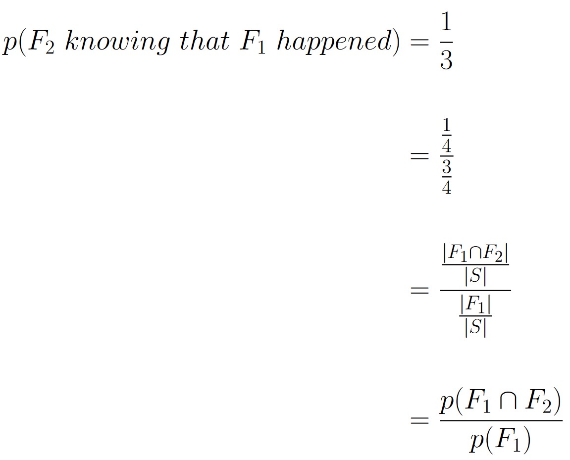
Reconsider the situation described in Example 2.1.2. Define the following events:

F₁:	“The showing face is black”
F₂:	“The hiding face is red”

The sample space S consists of the 4 possible faces, 3 of which are black, one of which is red, meaning |S| = 4. The probability that the hiding face is red, given that we know the face that is showing is black was calculated as follows:

Example 2.1.5

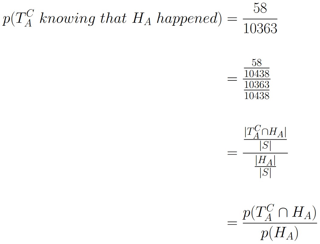
Consider the sample of aluminum cans described in Example 2.1.3.

Here, the sample space consisted of the 10438 cans taken by the engineer for quality assurance testing, so |S| = 10438.

Let’s define the following events:

T_A:	“The can’s wall thickness was acceptable”
H_A:	“The can’s height was acceptable”

First, we wanted to know how likely a can with acceptable height has problems with thickness. This would correspond to event T_A^C occurring knowing that event H_A occurred. We revisit that calculation below:

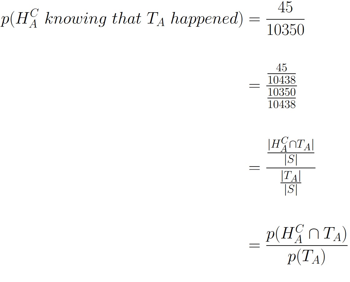
Next, we wanted to know how likely a can with acceptable thickness had any problems with height. That calculation is revisited and reexamined below:

We can start to see a pattern emerge the more we revisit the calculations we did previously.

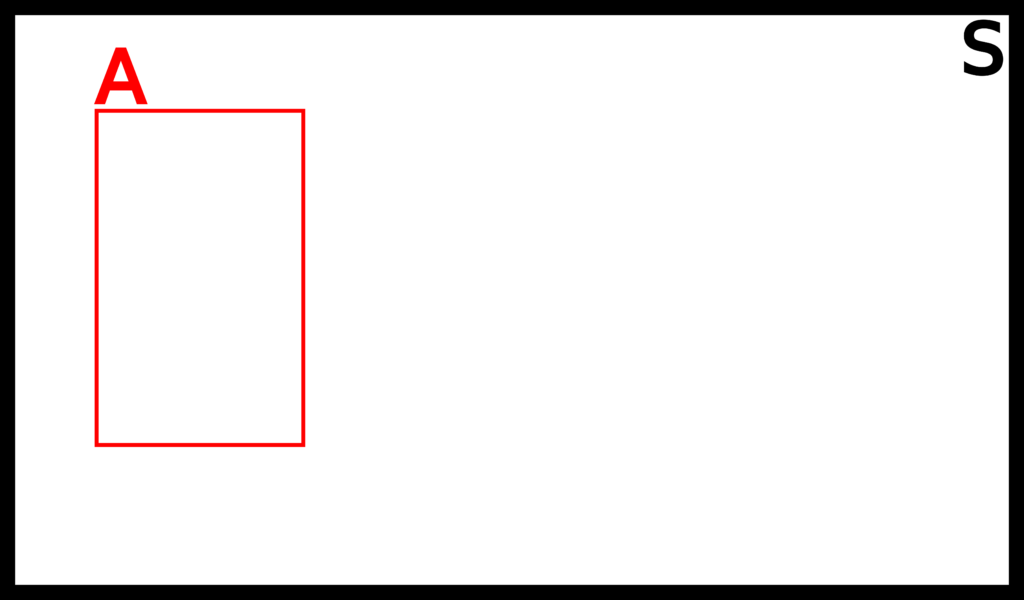
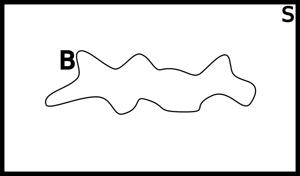
Figure 2.1.2: In (a) and (b) we show two events A and B respectively. The difference between “normal” probability and conditional probability can be demonstrated with (c) and (d). In (c), we calculate the probability of p(A∩B) as

In (d), we calculate the conditional probability p(A|B) by essentially ignoring anything in S that is not also in B. We then calculate p(A|B) as

Conditional Probability

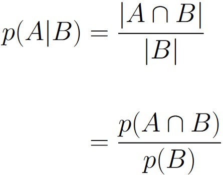
Suppose A and B are events within some sample space S. Furthermore, suppose

p(B) > 0.

We say that the conditional probability of event A occurring, given the fact that event B occurred is denoted

p(A | B),

and is defined as

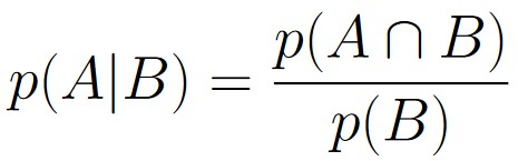
We can contextualize event B from the definition as being “extra information” that is supplied, and event A is the event we want to consider.

In Example 2.1.2, event B would correspond to the fact that the face showing up is black. The event A would correspond to the red face being hidden. Knowing that the displayed face is black changes the probability that the face being hidden is red because we have additional information that we did not have in Example 2.1.1.

Notice that the definition of conditional probability requires p(B) > 0. Of course, having p(B) = 0 would cause a division by zero, which is undefined. Furthermore, if p(B) = 0, then p(A ∩ B) would also be 0 since A ∩ B ⊆ B. This situation yields the indeterminate form 0/0. How do we interpret p(A|B) in this case? It’s hard to say, but this is why we require p(B) > 0 in the first place.

Example 2.1.6

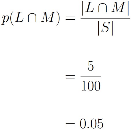
Suppose we’ve collected the following data regarding handedness:

	Left-Handed (L)	Right-Handed (R)	Totals
Male (M)	5	43	48
Female (F)	11	41	52
Totals	16	84	100

The sample includes data on 100 individuals, so |S| = 100. We can calculate the probability that a randomly selected person is a left-handed male like so:

Note that this is different then asking for the probability that a randomly selected male is left-handed. This is because we’re conditioning on the subject being a male. That means we ignore the female row and only consider the male row.

	Left-Handed (L)	Right-Handed (R)	Totals
Male (M)	5	43	48
Female (F)	11	41	52
Totals	16	84	100

As such, this is the probability p(L|M), which we calculate as follows:

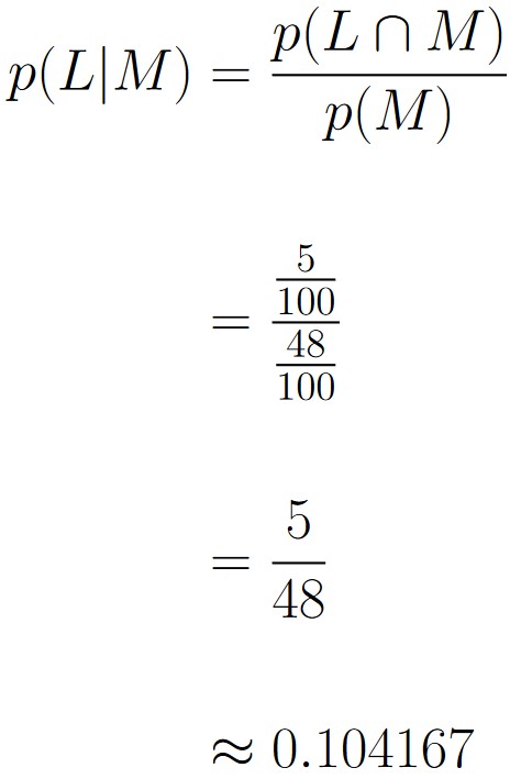
The probabilities p(L∩M) and p(L|M) are very different.