Physical Address
304 North Cardinal St.
Dorchester Center, MA 02124
Physical Address
304 North Cardinal St.
Dorchester Center, MA 02124
The axioms of probability are themselves surprisingly simple. The number of results we can derive from just three axioms is quite staggering.
In this section, we’ll build up a large arsenal of theorems we can use throughout this book, all derived from just those three axioms.
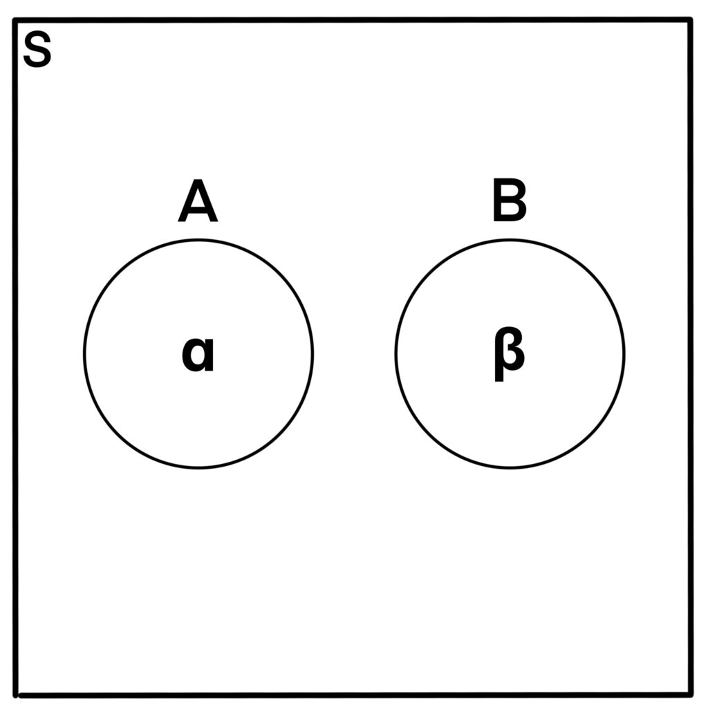
Figure 1.4.1: Consider a Venn Diagram with events A and B within sample space S. Here, α represents the proportion of the sample space taken up by event A, and β represents the proportion of the sample space taken up by event B. Since A and B are mutually exclusive, we can essentially take
α + β
to figure out how much of the sample space is taken up by
A ∪ B.
We can interpret p(A) and p(B) in a similar way. This gives us that
p(A ∪ B) = α + β = p(A) + p(B).
The probability of the null event (the empty set) is 0. In other words,
p(∅) = 0.
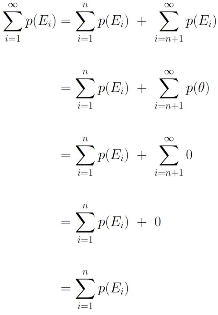
First, observe the fact that
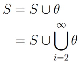
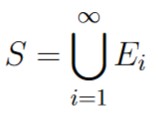
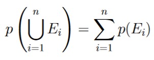
For any infinite collection of events Ei, let E1 = S, and for any i ≥ 2, let Ei = ∅. Therefore, Ei and Ej are mutually exclusive events when integers i and j are not equal. Therefore, we have that
Now, we can invoke Axiom 3:
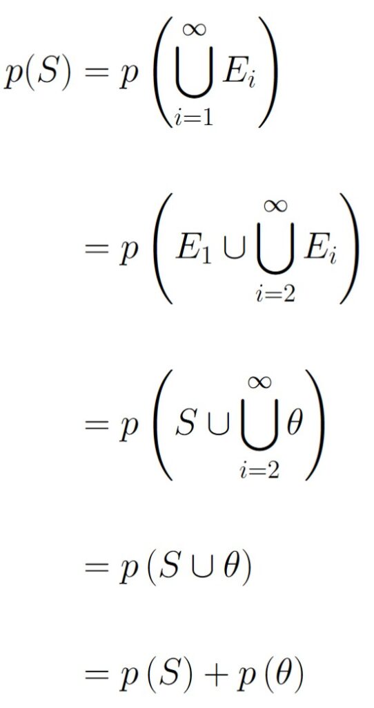
Now, we can invoke Axiom 2, which says that p(S) = 1, thus we have that
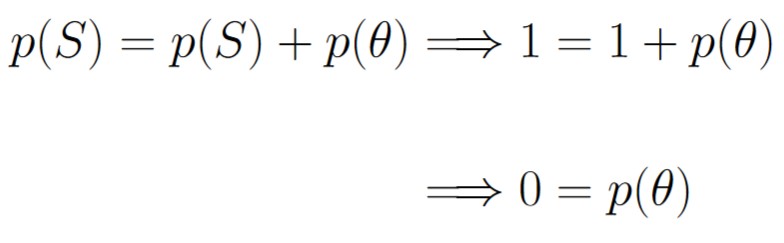
Which gives the result that p(∅) = 0 as desired.
For any finite collection {E1, E2, E3, E4, …, En} of mutually exclusive events taken from sample space S, we have that
 .
.
For all i > n, let Ei = ∅. Then, we get the following:
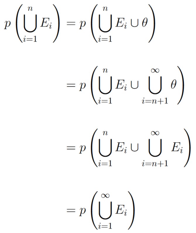
At this point, we can invoke Axiom 3:
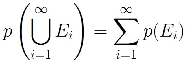
Now we can continue on by manipulating this sum as we need, making use of Theorem 1.4.1 along the way:
This gives us the desired result.
Theorem 1.4.2 means that we can essentially restrict Axiom 3 to a finite number of mutually exclusive events. We no longer have to deal with infinitely large collections of null events.
For some event E, we have that
p(EC) = 1 – p(E).
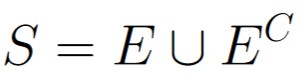
Consider an experiment with sample space S. For any event E, we have that
Invoking Theorem 1.4.2 yields the following:
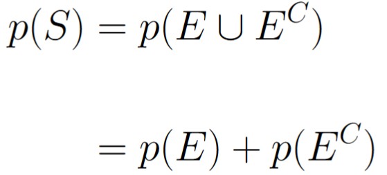
Now we can invoke Axiom 2:
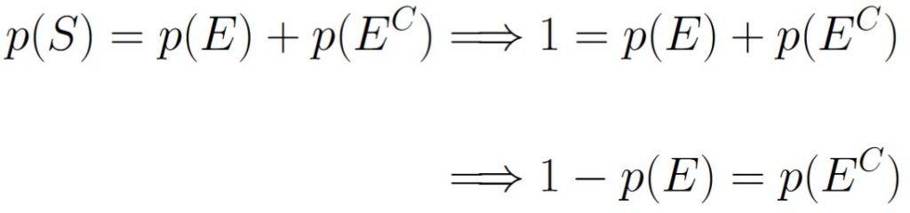
And so, we have that p(EC) = 1 – p(E) as desired.
Theorem 1.4.3, when combined with Axiom 1, gives us a lower bound and an upper bound on the probability of an event. For any event E from sample space S, we have that
0 ≤ p(E) ≤ 1
This inequality gives us a new definition for probability functions.
Consider an experiment with sample space S.
The probability function of the experiment, denoted p, is the function that assigns to each event from the sample space (each element of the sample space’s power set) a real number from [0, 1]. Symbolically, we write
p: P(S) → [0, 1].
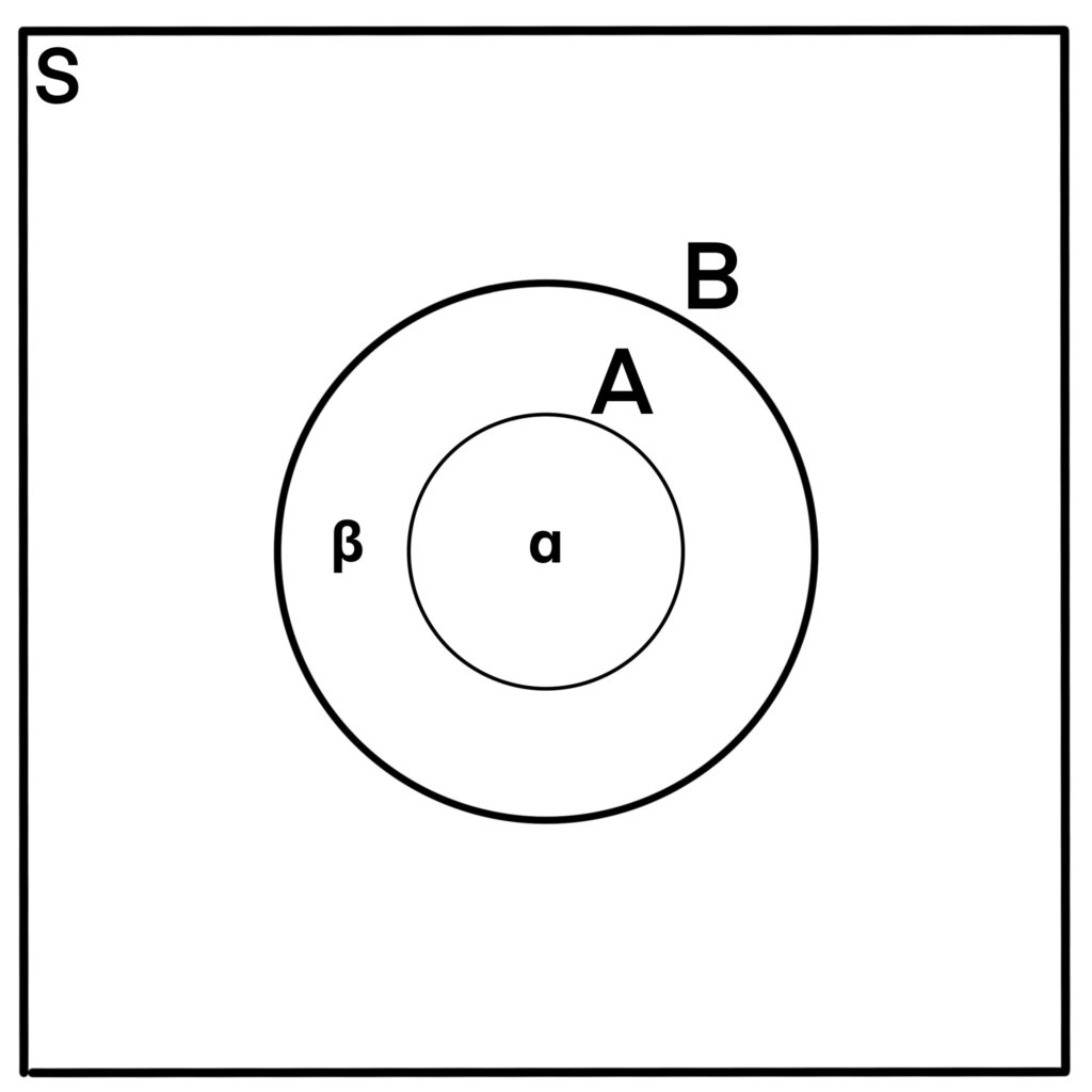
Figure 1.4.2: Here, event A is contained entirely within event B. In this scenario, the region marked by β does not include any part of the region marked by α. Event B corresponds to the sum α + β, whereas event A only corresponds to α. Thus, we essentially have that
p(B – A) = α + β – α = p(B) – p(A).
For any events A, B from sample space S with A ⊆ B, we have that
p(B – A) = p(B) – p(A).
The first thing we could do is to figure out what the complement of B – A is within S. We get the following:
Remember that since A ⊆ B, we have that BC ∩ A = ∅, meaning BC and A are mutually exclusive events within S. This means we can also invoke Theorem 1.4.2. Since we calculated the desired set’s complement, we can also invoke Theorem 1.4.3. We do this as follows:
Which gives us that p(B – A) = p(B) – p(A) as desired.
For any events A, B from sample space S with A ⊆ B, we have that
p(A) ≤ p(B).
We can utilize Axiom 1 and Theorem 1.4.5 as follows:
This gives us the desired result.
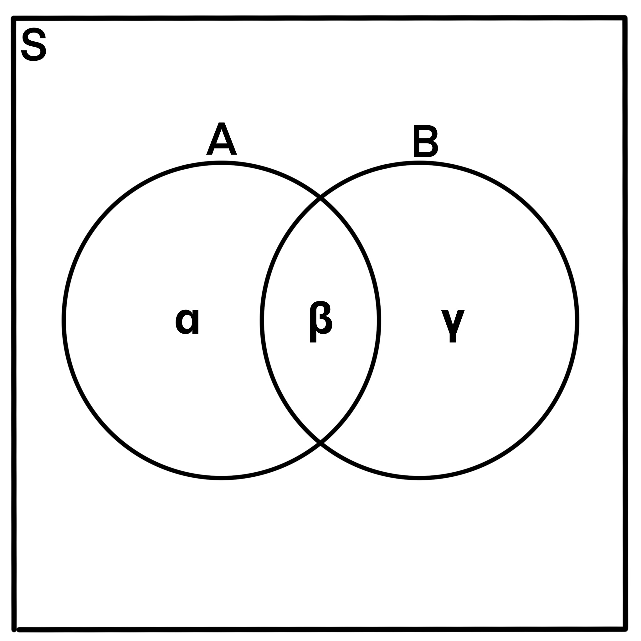
Figure 1.4.3: Notice that event A includes regions α and β, whereas event B includes regions β and γ. This gives us that
p(A) + p(B) = α + 2β + γ,
however, we clearly have that
p(A ∪ B) = α + β + γ.
Since
p(A ∩ B) = β,
we essentially have that
p(A ∪ B) = p(A) + p(B) – p(A ∩ B).
For any two events A and B from sample space S, we have that
p(A ∪ B) = p(A) + p(B) – p(A ∩ B).
Notice here, that we don’t know that A and B are mutually exclusive. Indeed there could be some overlap.
Instead, what we could do is recognize that events
A – (A ∩ B),
A ∩ B,
B – (A ∩ B)
are all mutually exclusive. Furthermore, we have that
A ∪ B = [A – (A ∩ B)] ∪ (A ∩ B) ∪ [B – (A ∩ B)].
We invoke Theorem 1.4.2 to get the following:
Now, we can use the fact that
A – (A ∩ B) ⊆ A
B – (A ∩ B) ⊆ B
along with Theorem 1.4.4 to get the following:
This completes the proof.
For any three events A, B, and C from sample space S, we have that
| p(A ∪ B ∪ C) | = | p(A) + p(B) + p(C) |
| – p(A ∩ B) – p(A ∩ C) – p(B ∩ C) | ||
| + p(A ∩ B ∩ C) |
We can basically just invoke Theorem 1.4.6 repeatedly. First, notice that
A ∪ B ∪ C = [A ∪ B] ∪ C,
which is just one way to associate the events together. The ensuing algebra gets a bit hairy, but is very doable with a little bit of patience and attention to detail. The algebra makes heavy use of the laws of set theory.
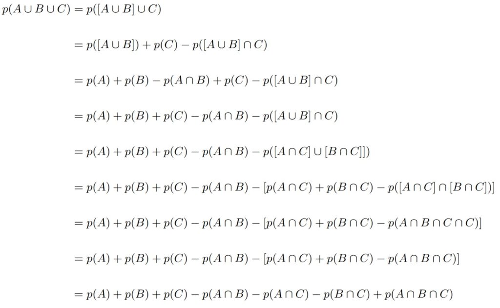
And finally, we have the desired result.
We could keep extending Theorem 1.4.7 to ever larger numbers of events. The key is to notice the pattern that emerges. Basically for any number of events, when we take events by an odd number at a time, we add. When we take events by an even number at a time, we subtract.
Of course, if you want to be pedantic and prove the formula for some number of events, you could keep using these theorems back to back (and recursively build up more “theorems”,) though that is usually unnecessary. Combinatorial arguments could be made to prove the most general form of Theorems 1.4.6 and 1.4.7, specifically, the Inclusion-Exclusion Principal.