Consider a hypothetical experiment where you are trying to pick a real number from the interval [-1, 2]. Clearly at this point, we have that |S| = [-1, 2].

Before we continue, we’ll define an equivalence relation on the interval [0, 1] by the following:

[0, 1]: x ~ y if x – y ∈ ℚ.

Basically, what this equivalence relation is saying is that for any two numbers x and y that are both in [0, 1], we say that x is related to y (symbolically, x ~ y) if x – y is a rational number. Because we’re dealing with an equivalence relation, we can examine some specific classes to get a better handle on what we’re dealing with.

Example 1.10.1

Consider the equivalence relation

[0, 1]: x ~ y if x – y ∈ ℚ.

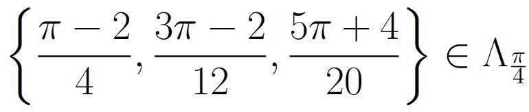
Suppose we want to know what numbers are related to . Using the language of equivalence relations, what we want to know is what numbers in [0, 1] are in the class .

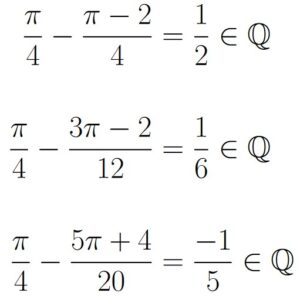
Some simple numbers we can try are other rational numbers:

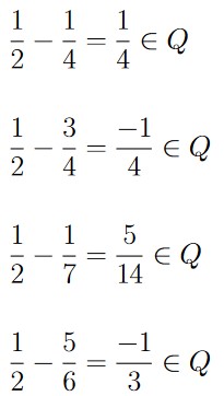
Which means that

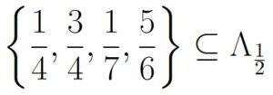
Notice that because

this tells us that

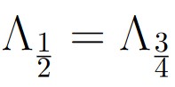
Of course, there are infinitely many numbers that are in the class , and as such all of those classes would be equal.

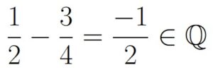
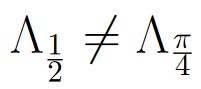
We can also use irrational numbers when looking for distinct classes, as in the following:

giving us that

Of course, these are two distinct classes because

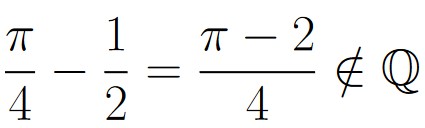
This gives us that

These are just two out of many examples of distinct classes we can list.

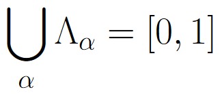
Note that because we have an equivalence relation on [0, 1], all of the distinct classes Λ_α form a partition of [0, 1]. As such, we have that

The reason we defined the equivalence relation on [0, 1] was to allow us to construct a very specific kind of subset, which we can refer to as E.

Before describing the construction, remember that ℚ is countably infinite, while ℝ is uncountably infinite. This means that each of the distinct classes that arise from our equivalence relation are countably infinite in cardinality (because they are defined to be all numbers that yield a rational number when subtracted from the number used to represent the class, and the rational numbers are countably infinite.) While each distinct class from the equivalence relation is countably infinite in cardinality, the number of distinct classes is uncountably infinite in cardinality because there are uncountably infinite possible numbers we can use to specify a class.

As a quick recap, remember that the while there are uncountably infinite classes in our equivalence relation, each of those classes themselves have a countably infinite number of elements.

Now, to define our subset E, consider each of the uncountably infinite number of classes Λ_α defined by our equivalence relation. From each of those classes, we are going to arbitrarily pick exactly one element. Our subset E of S is going to be the set of all of those arbitrarily picked elements. The Axiom of Choice guarantees the existence of this kind of set.

Example 1.10.2

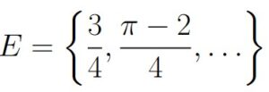
We just finished describing how E is going to be constructed, so let’s see an example of how E might look.

We know that , so we could pick an arbitrary point from both of those sets to be in E. For example, we might have

No other points from or are going to be in E.

Because there are an uncountably infinite number of classes, and E contains exactly one point from every single one of those distinct classes, E must be uncountably infinite in size. We now have a subset E that is a subset of S.

Now that we have constructed some subset E, let’s see what happens when we try to associate some kind of probability

p(E) = p_E.

with E.

Let’s start by defining some new sets that are related to E. First, define ℚ^{[-1, 1]} to be the set

ℚ^{[-1, 1]} = [-1, 1] ∩ ℚ,

or in other words, the set of all rational numbers in [-1, 1]. The reason for defining this set is that

x ∈ Λ_α ∧ y ∈ Λ_α ⟹ x – y ∈ [-1, 1] ∩ ℚ,

and so ℚ^{[-1, 1]} is a convenient short-hand.

Next, define E_n to be the set

E_n = { r_n + x : x ∈ E }

where r_n is the n^th number in ℚ^{[-1, 1]} (we can refer to the n^th number in ℚ^{[-1, 1]} since it is a subset of ℚ, a countably infinite set.) Basically, all we’re doing to define E_n is shifting all elements within E by some fixed amount r_n, a translation. This will essentially shift the interval of numbers from [0, 1] to [0 + r_n, 1 + r_n]. Based on how the equivalence relation is defined on [0, 1], and how ℚ^{[-1, 1]} was defined, we have that

[0 + r_n, 1 + r_n] ⊆ [-1, 2],

which is why S was defined to be the set [-1, 2] at the start of this section.

Because we’re assuming E is an event, we are also assuming that for all n ∈ ℕ, E_n is also an event. Furthermore, since E_n is a translation of E, we have that

p(E_n) = p(E) = p_E.

Now that we have defined a family of events that are all equally likely to occur, we can examine the consequences of defining E the way we did under the assumption that it is indeed an event (and thus has a probability.) Remember, in order for a subset to have a probability, we must satisfy the three axioms of probability theory.

We make two observations.

Observation 1: For all n ≠ m, E_n ∩ E_m = ∅

For any two distinct points x, y in E, we have that x – y ∉ ℚ. This is because all points from E come from distinct classes from the equivalence relation defined earlier. As such x + r_n ≠ y, no matter which n is chosen.

This means that for all n ≠ m, we have that x + r_n ≠ y + r_m. This means that

x ∈ E_n ⟺ x ∉ E_m.

Therefore, E_n ∩ E_m = ∅ whenever n ≠ m.

Observation 2: [0, 1] ⊆

Suppose we pick some x ∈ [0, 1].

By definition of E, there must then exist some y ∈ E such that x ~ y. By the equivalence relation defined earlier, this then means that x – y ∈ ℚ^{[-1, 1]}.

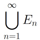
Put another way, there exists some n such that

x – y = r_n ⟹ x = y + r_n ⟹ x ∈ E_n ⟹ x ∈ .

To recap, we’ve just shown that

x ∈ [0, 1] ⟹ x ∈ .

This tells us that

[0, 1] ⊆ .

The Conclusion

Finally, note that because the interval [0, 1] has a length that is 1/3 of the length of [-1, 2], combining observations 1 and 2 together with Axiom 1 and Axiom 3 gives us the following:

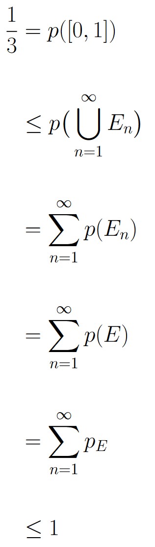
But, if we add the same number p_E ∈ [0, 1] to itself infinitely many times, the infinite sum is either 0 or ∞ (we know that if p_E is the probability of E occurring, then by the axioms of probability, we would have to have p_E ∈ [0, 1].)

This means that our original assumption that E is an event lead to a contradiction with the axioms of probability. Hence E must not be an event.