Physical Address
304 North Cardinal St.
Dorchester Center, MA 02124
Physical Address
304 North Cardinal St.
Dorchester Center, MA 02124

Understanding the laws of set theory is essential because they solve the problem of determining when two or more sets are equal through fundamental equations, including associativity, commutativity, and distribution. These laws provide a structured framework for defining and manipulating sets, ensuring consistency and precision in operations such as subset, difference, and symmetric difference.
In other words, by developing laws of set theory, we can essentially manipulate equations involving sets as if they were algebraic equations. In addition, the laws of set theory will allow us to convert complicated expressions involving sets into simpler ones, much like how we took complicated logical expressions, and simplified them into smaller, logically equivalent expressions.
By studying these laws, one can formulate and prove mathematical concepts and theorems accurately. Furthermore, the foundations of many branches of mathematics are developed using the language of sets and set theory. In addition to the further development of mathematics, these laws will also prove crucial crucial to subjects like computer science and data science.
We have briefly described some aspects of set equality when we first introduced what sets were. We talked about how repetition and order are irrelevant with respect to what elements are contained within a set. As such, even if some elements are repeated in various elements, they still represent the same set.
However, as we have also seen, there are a wide variety of methods to describe a set and what elements are contained within. Just because we come up with different descriptions, that does not necessarily mean we are describing different sets, but sometimes we may be describing exactly the same set.
Consider the set
M = { x | x is an even number between -3 and 10 inclusive }.
Of course, we already know what elements are in M:
M = { -2, 0, 2, 4, 6, 8, 10 }.
Now consider the set
N = { 4x + 3 | x ∈ {-1.25, -0.75, -0.25, 0.25, 0.75, 1.25, 1.75} }.
The description of N is a little more complicated, but we can still determine what elements are in N. The only tricky part is recognizing that the elements of N are based of elements that are in the set
{-1.25, -0.75, -0.25, 0.25, 0.75, 1.25, 1.75},
so we just have to iterate over those elements to figure out what is in N. We’ll tabulate all values below:
| x | 4x | 4x + 3 |
|---|---|---|
| -1.25 | -5 | -2 |
| -0.75 | -3 | 0 |
| -0.25 | -1 | 2 |
| 0.25 | 1 | 4 |
| 0.75 | 3 | 6 |
| 1.25 | 5 | 8 |
| 1.75 | 7 | 10 |
Since N consists of the values 4x + 3, we now know that
N = { -2, 0, 2, 4, 6, 8, 10 }.
Notice that M and N have the same number of elements (7), and all elements are exactly the same. Thus, since M and N represent the exact same set, we could write
M = N.
It’s worth pointing out that since every element in M is also in N, and that every element in N is also in M, we have that
| M ⊆ N | N ⊆ M |
However, defining set equality by having the same elements is not exactly rigorous. Two sets can share some number of elements, while also having different elements. As such, we don’t define set equality by simply having the same elements. Instead, we look to the end of Example 3.5.1 for inspiration.
Consider the two sets A and B taken from some universal set 𝒰.
Sets A and B are called equal, and we write A = B when
A ⊆ B
and
B ⊆ A.
This definition is precise because we can determine if a set is a subset of another set under scrutiny. As such, because the definition of set equality requires we show two things to be true, proofs showing two sets to be equal are usually broken up into two parts.
It’s this definition of set equality that makes the next two theorems somewhat straight-forward to prove.
For any A, B ⊆ 𝒰 (that is, sets A and B are both subsets of 𝒰), if A ⊆ B, then A ∩ B = A.
Step 1: Show that A ∩ B ⊆ A
Let x be an arbitrarily picked element within A ∩ B (meaning x ∈ A ∩ B.)
By definition, x ∈ A and x ∈ B, and as such we know that x ∈ A.
Thus, we have shown that if x ∈ A ∩ B, then x ∈ A. This means that A ∩ B ⊆ A, completing step 1.
Step 2: Show that A ⊆ A ∩ B
Let x be an arbitrarily picked element of A. Because we have by premise that A ⊆ B, we also have that x ∈ B.
Thus, since x ∈ A and x ∈ B, we have that x ∈ A ∩ B by definition.
We have just shown that when x ∈ A, we also have that x ∈ A ∩ B. We then have by definition that A ⊆ A ∩ B, completing step 2.
Conclusion
Because we have shown that A ⊆ A ∩ B and that A ∩ B ⊆ A, we have by definition that
A ∩ B = A
as desired.
Thus, by Theorem 3.5.1, whenever we know that A ⊆ B, we can replace A ∩ B with just A anytime we see A ⊆ B in an equation.It’s worth stressing that we can only make such a replacement when we know A ⊆ B. Otherwise, doing so may not be correct.
There are a few more such equalities we can make use of, which we now show in the next theorem.
For any A, B ⊆ 𝒰, we have that
| A ⊆ B | ⟺ | A ∩ B = A | ⟺ | A ∪ B = B | ⟺ | BC ⊆ AC |
We’ll break this proof up into 4 steps.
Step 1: A ⊆ B ⟹ A ∩ B = A
This is simply Theorem 3.5.#.
Step 2: A ∩ B = A ⟹ A ∪ B = B
The premise of this logical implication is that A ∩ B = A, so we can bring that fact in whenever needed.
First we show that A ∪ B ⊆ B.
Let x be an arbitrarily picked element in A ∪ B. Thus, by definition x ∈ A or x ∈ B. If x happens to be an element of B, then it is tautologically true that x ∈ B.
If x ∈ A, then the premise tells us that x ∈ A ∩ B, meaning x ∈ B as well.
Either way, we have that whenever x ∈ A ∪ B, we also have that x ∈ B, meaning A ∪ B ⊆ B.
Second, we show that B ⊆ A ∪ B.
Let x be an arbitrarily picked element within B. Thus, because x ∈ B, we also have that x ∈ A ∪ B.
Thus, we have just shown that whenever x ∈ B, we also have that x ∈ A ∪ B. This means that B ⊆ A ∪ B.
Finally, because we have shown that A ∪ B ⊆ B and B ⊆ A ∪ B, we have that
A ∪ B = B
as desired.
Step 3: A ∪ B = B ⟹ BC ⊆ AC
Remember that AC is the complement of A within 𝒰. Also remember that A ∪ B = B is a premise of this logical implication, so we can use that fact whenever we want (we can’t use A ∩ B = A as a premise here, since that is not included in the implication we are considering.)
We are trying to show that BC ⊆ AC, so let x be an arbitrarily picked element of BC.
Because x ∈ BC, we have by definition that x ∉ B. Now, because A ∪ B = B and x ∉ B, we also have that x ∉ A ∪ B.
Next, because x ∉ A ∪ B, we also know that x ∉ A. Therefore, since x ∉ A, we must have that x ∈ AC.
We have just shown that whenever x ∈ BC, we also have that x ∈ AC (assuming A ∪ B = B as a premise.)
Thus by definition, whenever we know A ∪ B = B, we have that BC ⊆ AC as desired.
Step 4: BC ⊆ AC ⟹ A ⊆ B
We have BC ⊆ AC as a premise, so we’ll invoke that fact when needed.
Let x be an arbitrarily picked element of A. Since x ∈ A, we have by definition that x ∉ AC.
Now, because BC ⊆ AC and x ∉ AC, we have (by Modus Tollens) that x ∉ BC.
Now, because x ∉ BC, we have by definition that x ∈ B.
Thus, we have shown that, assuming BC ⊆ AC as a premise, whenever x ∈ A, we must also have that x ∈ B.
Therefore, assuming BC ⊆ AC as a premise, we have that A ⊆ B as desired.
Conclusion
Because we have shown that
| A ⊆ B | ⟹ | A ∩ B = A |
| A ∩ B = A | ⟹ | A ∪ B = B |
| A ∪ B = B | ⟹ | BC ⊆ AC |
| BC ⊆ AC | ⟹ | A ⊆ B |
We have that they are all logically equivalent, meaning we have that
| A ⊆ B | ⟺ | A ∩ B = A | ⟺ | A ∪ B = B | ⟺ | BC ⊆ AC |
as desired.
Because of Theorem 3.5.2, whenever we know one of
| A ⊆ B | A ∩ B = A | A ∪ B = B | BC ⊆ AC |
are true, we automatically know that the other 3 are true as well.
The total opposite of two sets A and B being equal, is when A and B have absolutely no elements in common. Of course, if two sets share no element in common, then their intersection is a set that has no elements in it, which is just the empty set.
Consider the two sets A and B taken from some universal set 𝒰.
A and B are called disjoint whenever
A ∩ B = ∅.
Many of the concepts discussed so far may seem disparate. However, they are more connected than may initially appear.
Let A, B ⊆ 𝒰.
A ∩ B = ∅ ⟺ A ∪ B = A △ B
Because we have a logical biconditional, we break this proof into two steps. First, we assume A ∩ B = ∅ as a premise and show that A ∪ B = A △ B.
Next, we assume A ∪ B = A △ B as a premise and show that A ∩ B = ∅.
Step 1: A ∩ B = ∅ ⟹ A ∪ B = A △ B
First, we try to show that A ∪ B ⊆ A △ B.
Let x be an arbitrarily picked element within A ∪ B. Thus, we have by definition that x ∈ A or x ∈ B, but because A ∩ B = ∅, x can’t be in both A and B.
Thus we either have that x ∈ A and x ∉ B, meaning x ∈ A △ B, or we have that x ∉ A and x ∈ B, meaning we still have that x ∈ A △ B.
Either way, we have that x ∈ A △ B. Hence, we just shown that (assuming A ∩ B = ∅) whenever x ∈ A ∪ B, we also have that x ∈ A △ B as well, and so we have that
A ∪ B ⊆ A △ B.
Second, we try to show that A △ B ⊆ A ∪ B.
Now, let x be an arbitrarily picked element in A △ B. Thus, by definition, either x ∈ A and x ∉ B, meaning x ∈ A ∪ B, or x ∉ A and x ∈ B, meaning x ∈ A ∪ B.
Either way, we know that whenever x ∈ A △ B, we also know that x ∈ A ∪ B as well.
Thus, by definition we have that
A △ B ⊆ A ∪ B.
Finally, because we know that A ∪ B ⊆ A △ B and A △ B ⊆ A ∪ B, we have by definition that
A ∪ B = A △ B.
Thus, whenever we know that A and B are disjoint (A ∩ B = ∅), we know that A ∪ B = A △ B.
This shows that A ∩ B = ∅ ⟹ A ∪ B = A △ B, completing step 1.
Step 2: A ∩ B = ∅ ⟸ A ∪ B = A △ B
Here, we are assuming A ∪ B = A △ B as a premise, and are trying to show that A ∩ B = ∅.
Because we know that A ∪ B = A △ B, we have by definition of set equality that A ∪ B ⊆ A △ B and A △ B ⊆ A ∪ B, and so A ∪ B ⊆ A △ B.
Thus, for any element x ∈ A ∪ B, we also know that x ∈ A △ B. However, since x ∈ A △ B, we know that either
| x ∈ A and x ∉ B | or | x ∉ A and x ∈ B |
Either way, no element x ∈ A ∪ B can be in both A and B.
Thus, because no element x exists such that x ∈ A ∩ B, we must have that A ∩ B is empty, meaning A ∩ B = ∅.
This shows that A ∪ B = A △ B ⟹ A ∩ B = ∅, completing step 2.
Conclusion
Because we’ve shown that
A ∩ B = ∅ ⟹ A ∪ B = A △ B
and
A ∪ B = A △ B ⟹ A ∩ B = ∅
we must have that
A ∩ B = ∅ ⟺ A ∪ B = A △ B
as desired.
Theorem 3.5.3 connects the concepts of equal sets, disjoint sets, unions, and symmetric differences.
Remember that
x ∈ A
is a statement about x being a member of set A. Because it is a statement, it has a truth value of either 0 or 1.
One powerful tool we had at our disposal for analyzing logical expressions was a truth table. We can adapt truth tables to analyze set relationships as well. In this case, membership tables offer a tabular way of representing element arguments.
| x ∈ A | x ∈ B | x ∈ A ∪ B | x ∈ A ∩ B |
|---|---|---|---|
| 0 | 0 | 0 | 0 |
| 0 | 1 | 1 | 0 |
| 1 | 0 | 1 | 0 |
| 1 | 1 | 1 | 1 |
Instead of using some generic symbol for a generic object whose membership in some set we want to analyze, we could simply list whatever sets we’re analyzing. As such, we could rewrite the above table like so:
| A | B | A ∪ B | A ∩ B |
|---|---|---|---|
| 0 | 0 | 0 | 0 |
| 0 | 1 | 1 | 0 |
| 1 | 0 | 1 | 0 |
| 1 | 1 | 1 | 1 |
All of the set operations have their corresponding tables, which we can include inside one large table, like the one below:
| AC | ¬a |
| A ∪ B | a ∨ b |
| A ∩ B | a ∧ b |
| A – B | ¬(a → b) |
| A △ B | a ⊻ b |
Figure 3.5.1: Based on the values presented in Table 3.5.1, we see that there are obvious analogues with logical operators. The above table lists them. Notice that the set difference resembles the logical complement of an implication.
| A | B | AC | A ∪ B | A ∩ B | A – B | A △ B |
|---|---|---|---|---|---|---|
| 0 | 0 | 1 | 0 | 0 | 0 | 0 |
| 0 | 1 | 1 | 1 | 0 | 0 | 1 |
| 1 | 0 | 0 | 1 | 0 | 1 | 1 |
| 1 | 1 | 0 | 1 | 1 | 0 | 0 |
Table 3.5.1: Here is a membership table for all of the major set operations.
In addition to the set operations, we can determine subset relationships. Let’s take a look at one more table to see some kind of example:
| x ∈ A | x ∈ B | x ∈ A ∪ B | x ∈ A ∩ B | x ∈ A ∩ B → x ∈ A | x ∈ A → x ∈ A ∪ B |
|---|---|---|---|---|---|
| 0 | 0 | 0 | 0 | 1 | 1 |
| 0 | 1 | 1 | 0 | 1 | 1 |
| 1 | 0 | 1 | 0 | 1 | 1 |
| 1 | 1 | 1 | 1 | 1 | 1 |
Notice that the columns
| x ∈ A ∩ B → x ∈ A | x ∈ A → x ∈ A ∪ B |
have all 1s. As such, we can write
| x ∈ A ∩ B ⟹ x ∈ A | x ∈ A ⟹ x ∈ A ∪ B |
which is exactly the definition of subset. As such, we can determine that a set A is a subset of some other set B by comparing their respective columns. If A has 1s in all rows where B has 1s, then we know that A ⊆ B.
Let’s prove a simple observation we may have had in our study of set relationships and operations.
Let A, B ⊆ 𝒰.
(A ∩ B) ⊆ A ⊆ (A ∪ B)
Let’s examine a membership table:
| A | B | A ∪ B | A ∩ B |
|---|---|---|---|
| 0 | 0 | 0 | 0 |
| 0 | 1 | 1 | 0 |
| 1 | 0 | 1 | 0 |
| 1 | 1 | 1 | 1 |
Now, we can compare specific columns we want, but we’ll do so in two separate membership tables:
| A ∩ B | A |
|---|---|
| 0 | 0 |
| 0 | 0 |
| 0 | 1 |
| 1 | 1 |
| A | A ∪ B |
|---|---|
| 0 | 0 |
| 0 | 1 |
| 1 | 1 |
| 1 | 1 |
Notice that in the above table on the left, every row of A ∩ B that has a 1 also has a 1 in the A column. As such, we know that (A ∩ B) ⊆ A.
Additionally, from the table above on the right, every row in the A column that has a 1 also has a 1 in the A ∪ B column. As such, we know that A ⊆ (A ∪ B).
Because we know that (A ∩ B) ⊆ A and A ⊆ (A ∪ B), we can combine them into the single expression
(A ∩ B) ⊆ A ⊆ (A ∪ B)
as desired.
Membership tables can be a convenient way to represent an element argument in tabular form. However, membership tables will not totally replace element arguments, as sometimes, the element argument is simpler to make for more esoteric situations where tables can be cumbersome to use.
We’ve already examined a number of some simple laws (referred to as theorems) above, and have demonstrated their truth by way of element arguments and membership tables. What’s demonstrated above only scratches the surface of the multitude of equal set relationships we can exploit. Below, we present a large table offering even more such laws.
As you look over this table, it would be wise to compare this table with the table presented in Chapter 1, Section 4. You should see many analogues.
For any sets A, B, and C taken from some universal set C, we have the following equivalencies:
| (AC)C = A | Law of Double Complement |
| (A ∪ B)C = AC ∩ BC (A ∩ B)C = AC ∪ BC | DeMorgan’s Laws |
| A ∪ B = B ∪ A A ∩ B = B ∩ A | Commutative Laws |
| A ∪ (B ∪ C) = (A ∪ B) ∪ C A ∩ (B ∩ C) = (A ∩ B) ∩ C | Associative Laws |
| A ∪ (B ∩ C) = (A ∪ B) ∩ (A ∪ C) A ∩ (B ∪ C) = (A ∩ B) ∪ (A ∩ C) | Distributive Laws |
| A ∪ A = A A ∩ A = A | Idempotent Laws |
| A ∪ ∅ = A A ∩ 𝒰 = A | Identity Laws |
| A ∪ AC = 𝒰 A ∩ AC = ∅ | Inverse Laws |
| A ∪ 𝒰 = 𝒰 A ∩ ∅ = ∅ | Domination Laws |
| A ∪ (A ∩ B) = A A ∩ (A ∪ B) = A | Absorption Laws |
Table 3.5.2: Here is a large table laying out various set equivalencies, which we refer to as the laws of set theory.
Certainly, many more such laws and equivalencies exist, but the above table represents some of the more ubiquitous laws that are often used.
These laws present us an opportunity to directly compare three different proof techniques. First, we use a membership table.
For any A ⊆ 𝒰,
(AC)C = A
General Strategy: we’ll use a membership table to compare the columns for A and (AC)C.
| A | AC | (AC)C |
|---|---|---|
| 0 | 1 | 0 |
| 1 | 0 | 1 |
Since the columns for A and (AC)C are exactly the same, they are equal, and so we have
A = (AC)C
as desired.
Now, compare such a simple strategy with a standard element argument used in the next proof.
For any A, B ⊆ 𝒰,
(A ∪ B)C = AC ∩ BC
(A ∩ B)C = AC ∪ BC
General Strategy: we’ll split this proof up into two steps, where each step will be dedicated to each different part of DeMorgan’s Laws. Both steps will make use of standard element arguments, as well as the definition of set equality.
Step 1: (A ∪ B)C = AC ∩ BC
First, we show that (A ∪ B)C ⊆ AC ∩ BC
First, suppose that element x ∈ 𝒰 was also in (A ∪ B)C, meaning x ∈ (A ∪ B)C.
Since, x ∈ (A ∪ B)C, we know that x ∉ ((A ∪ B)C)C, and by the Law of Double Complement, we also know that x ∉ A ∪ B.
Now we simultaneously know that x ∉ A (otherwise x would be in A ∪ B, which we just established was not the case) and x ∉ B (again, because then x would be in A ∪ B.)
Thus, since x ∉ A and x ∉ B, we know that x ∈ AC and x ∈ BC, meaning x ∈ AC ∩ BC, which is what we’re trying to show.
Thus, whenever we have that x ∈ (A ∪ B)C, we know that x ∈ AC ∩ BC, meaning
(A ∪ B)C ⊆ AC ∩ BC.
Second, we show that AC ∩ BC ⊆ (A ∪ B)C.
Now, suppose we knew that x ∈ AC ∩ BC. Thus we simultaneously know that x ∈ AC and x ∈ BC.
This means we have that x ∉ A and x ∉ B. Thus, since x is in neither A nor B, x can’t possibly be in A ∪ B, meaning x ∉ A ∪ B. This means that x ∈ (A ∪ B)C.
Thus, whenever we know that x ∈ AC ∩ BC, we also know that x ∈ (A ∪ B)C which means we have that
AC ∩ BC ⊆ (A ∪ B)C.
Finally, because we’ve shown that (A ∪ B)C ⊆ AC ∩ BC and AC ∩ BC ⊆ (A ∪ B)C, we have by definition that
(A ∪ B)C = AC ∩ BC
as desired.
Step 2: (A ∩ B)C = AC ∪ BC
Using nearly the exact same process as was used in step 1, we come to the conclusion that
(A ∪ B)C = AC ∩ BC.
Conclusion
By now, we have shown that both
(A ∪ B)C = AC ∩ BC
and
(A ∩ B)C = AC ∪ BC
and as such have completely established DeMorgan’s Laws.
The last of these laws we’ll prove in this section will be the Distributive Laws. Instead of making two separate element arguments to establish that A ∪ (B ∩ C) ⊆ (A ∪ B) ∩ (A ∪ C) and (A ∪ B) ∩ (A ∪ C) ⊆ A ∪ (B ∩ C), we will use logical equivalencies to show that A ∪ (B ∩ C) and (A ∪ B) ∩ (A ∪ C) are subsets of each other simultaneously.
For any A, B, C ⊆ 𝒰,
A ∪ (B ∩ C) = (A ∪ B) ∩ (A ∪ C)
A ∩ (B ∪ C) = (A ∩ B) ∪ (A ∩ C)
General Strategy: we’ll use logical equivalencies to show that any element of A ∪ (B ∩ C) is also an element of (A ∪ B) ∩ (A ∪ C). Since we use logical equivalencies, this also applies the other way simultaneously.
| x ∈ A ∪ (B ∩ C) | Starting Proposition | |
| ⟺ | (x ∈ A) ∨ (x ∈ B ∩ C) | Definition of Set Union |
| ⟺ | (x ∈ A) ∨ [(x ∈ B) ∧ (x ∈ C)] | Definition of Set Intersection |
| ⟺ | [(x ∈ A) ∨ (x ∈ B)] ∧ [(x ∈ A) ∨ (x ∈ C)] | Distribution of ∨ over ∧ |
| ⟺ | [x ∈ A ∪ B] ∧ [x ∈ A ∪ C] | Definition of Set Union |
| ⟺ | x ∈ (A ∪ B) ∩ (A ∪ C) | Definition of Set Intersection |
We have just established that
x ∈ A ∪ (B ∩ C) ⟺ x ∈ (A ∪ B) ∩ (A ∪ C).
Thus, whenever x ∈ A ∪ (B ∩ C), we also simultaneously know that x ∈ (A ∪ B) ∩ (A ∪ C). As such, we know that
| A ∪ (B ∩ C) ⊆ (A ∪ B) ∩ (A ∪ C) | (A ∪ B) ∩ (A ∪ C) ⊆ A ∪ (B ∩ C) |
are simultaneously true, and so we have that
A ∪ (B ∩ C) = (A ∪ B) ∩ (A ∪ C)
as desired.
The same logic also works to tell us that
A ∩ (B ∪ C) = (A ∩ B) ∪ (A ∩ C)
as well.
Of course, the rest of the Laws of Set Theory can be be proven in many different ways. Because it is a good exercise to provide a proof for all the above laws, proofs for the remaining laws are asked for in this chapter’s practice questions.
Just as we can use the Laws of Logic to simplify complicated logical expressions, we can also use the Laws of Set Theory to simplify complicated expressions involving sets.
Suppose we were dealing with the expression
X ∩ (Y – X)
where X, Y ⊆ 𝒰.
We can simplify the above expression in the following way:
| X ∩ (Y – X) | Starting Expression | |
| ⟺ | X ∩ (Y ∩ XC) | Definition of Set Difference |
| ⟺ | X ∩ (XC ∩ Y) | Commutative Law |
| ⟺ | (X ∩ XC) ∩ Y | Associative Law |
| ⟺ | ∅ ∩ Y | Inverse Law |
| ⟺ | ∅ | Domination Law |
Thus, we have just established that for any X, Y ⊆ 𝒰,
X ∩ (Y – X) = ∅.
For any two sets A and B taken from some universal set 𝒰, we have that
A – B = A ∩ BC
Figure 3.5.2: We can express the operation of set difference using only union, intersection, and complement.
We did make use of a fact (an additional law of Set Theory) where we can express the set difference operation using only intersection and complement:
Y – X = Y ∩ XC.
We will now justify that equality:
| Y – X | Starting Expression | |
| = | { p | p ∈ Y ∧ p ∉ X } | Definition of Set Difference |
| = | { p | p ∈ Y ∧ p ∈ XC } | Definition of Set Complement |
| = | Y ∩ XC | Definition of Set Intersection |
For any two sets A and B taken from some universal set 𝒰, we have that
A △ B = (A ∩ BC) ∪ (BC ∩ A)
Figure 3.5.3: We can express the Symmetric Difference operation using only union, intersection, and complement
As a matter of fact, we can also express the Symmetric Difference operation using only union, intersection, and complement operators as well, which we justify below:
| Y △ X | Starting Expression | |
| = | { p | p ∈ Y ⊻ p ∈ X } | Definition of Symmetric Difference |
| = | { p | (p ∈ Y ∧ p ∉ X) ∨ (p ∉ Y ∧ p ∈ X) } | Definition of Logical Exclusive-or |
| = | { p | (p ∈ Y ∧ p ∈ XC) ∨ (p ∈ YC ∧ p ∈ X) } | Definition of Set Complement |
| = | { p | (p ∈ Y ∩ XC) ∨ (p ∈ YC ∩ X) } | Definition of Set Intersection |
| = | (Y ∩ XC) ∪ (YC ∩ X) | Definition of Set Union |
This just goes to show how important the Union, Intersection, and Complement operations are when it comes to sets, because no matter how we want to combine any combination of sets, we can always do so using just those three operations.
Can we rewrite the expression
(X – Y)C
using only Union, Intersection, and Complement? Let’s try and see.
| (X – Y)C | Starting Expression | |
| = | (X ∩ YC)C | Definition of Set Difference |
| = | XC ∪ (YC)C | DeMorgan’s Law |
| = | XC ∪ Y | Law of Double Complement |
So (X – Y)C is equivalent to XC ∪ Y.
We can simplify the expression
(((X ∪ Y) ∩ Z)C ∪ Y)C
using the following steps:
| (((X ∪ Y) ∩ Z)C ∪ Y)C | Starting Expression | |
| = | (((X ∪ Y) ∩ Z)C)C ∩ (YC)C | DeMorgan’s Law |
| = | ((X ∪ Y) ∩ Z) ∩ Y | Law of Double Complement |
| = | (Z ∩ (X ∪ Y)) ∩ Y | Commutative Law |
| = | Z ∩ ((X ∪ Y)) ∩ Y) | Associative Law |
| = | Z ∩ ((X ∩ Y) ∪ (Y ∩ Y)) | Distributive Law |
| = | Z ∩ ((X ∩ Y) ∪ Y) | Idempotent Law |
| = | Z ∩ (Y ∪ (X ∩ Y)) | Associative Law |
| = | Z ∩ Y | Absorption Law |
We’ve seen DeMorgan’s Laws applied to two sets at a time. Let’s see what happens when we have three sets at a time:
| (A ∪ B ∪ C)C | Starting Expression | |
| = | ((A ∪ B) ∪ C)C | Associative Law |
| = | (A ∪ B)C ∩ CC | DeMorgan’s Laws |
| = | AC ∩ BC ∩ CC | DeMorgan’s Law |
It stands to reason that repeated applications of DeMorgan’s Laws would work for intersection as well.
Furthermore, no matter how many sets we have, it seems as if we can just repeatedly apply DeMorgan’s Laws and the Associative Law. Based on this observation, we make the following observations:
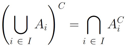
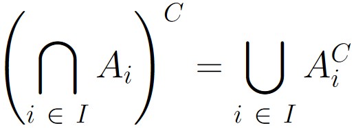
Figure 3.5.4: Above are depicted the generalized versions of DeMorgan’s Laws. In (a), we see the general version of taking the complement of a multiple union. In (b), we see a general version of taking the complement of a multiple intersection.
In Figure 3.5.4, I is an index set over which the multiple union or intersection is taken.
Of course, mere intuition doesn’t prove anything to be true. Instead, we must rely on rigorous tools, such as element arguments and logical equivalencies, to establish truth without any doubt.
For a universal set 𝒰 and index set I, the following equalities hold:
General Strategy: we’ll make use of various definitions of Set Theory, including Complement. We also make use of the logical rules that apply when negating quantified statements as discussed in Chapter 1, Section 9.
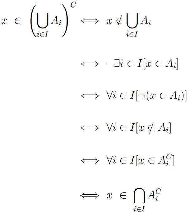
We’ve just shown why the equivalence in (a) is true. By similar logic, part (b) is also shown to be true. This establishes both equivalencies as desired.
The generalized versions of DeMorgan’s Laws will prove extremely useful in our further study of math.