Physical Address
304 North Cardinal St.
Dorchester Center, MA 02124
Physical Address
304 North Cardinal St.
Dorchester Center, MA 02124

We’ve seen two examples of logically equivalent expressions. For example, on this page, we verified that
¬(p ∧ q) ⇔ ¬p ∨¬q
¬(p ∨ q) ⇔ ¬p ∧¬q
These two sets of equivalencies are known as DeMorgan’s Laws. We’ve also seen that
p ∧ (q ∨ r) ⇔ (p ∧ q) ∨ (p ∧ r)
p ∨ (q ∧ r) ⇔ (p ∨ q) ∧ (p ∨ r)
These two sets of equivalencies are known as the distributive laws.
Throughout this page, we’ll see many more kinds of these logical equivalencies.
Is there a statement that is logically equivalent to
¬(¬p ∨ q)
but simpler?
The first thing we may do is construct a truth table. Using Maple (as discussed in this chapter’s Maple section,) we get the following:
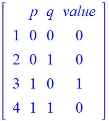
So, it looks like our expression is only equal to 1 when p = 1 and q = 0.
Thinking back to the definitions of connectives, we may notice that this expression almost looks like p ∧ q. The only difference is that the 1 moved up a row.
Looking at the columns for p and q, we notice that the only place where two 1s line up is in the fourth row. If we want to use ∧, then we need the second 1 in the q column to move up one row. We can do this by negating q.
Great, so we have the exact same truth values for p ∧ ¬q as ¬(¬p ∨ q). This means that
¬(¬p ∨ q) ⇔ p ∧ ¬q
as desired.
This second expression has one fewer negation, and lacks parenthesis, so our new expression is simpler than the given expression.
We could also notice that this new expression is also logically equivalent to ¬(p → q), though this doesn’t seem as simple as p ∧ ¬q, mainly because there’s a negation outside of the parenthesis.
The solution we came up with for Example 1.4.1 required us to make a keen observation about how to line up the 1s and 0s in a truth table to get the desired outcome. It would be nice if we had a more systematic way of coming up with logically equivalent statements, though we’ll probably never get to a point where detailed analysis can be eschewed. Nevertheless, we can make the process somewhat easier.
As discussed on this page, any two logically equivalent statements s1 and s2 have the exact same truth values. This means that when we see s1 in a logical expression, we can replace it with s2 and not change the truth value of the overall logical expression.
Here is a big list of logically equivalent expressions, all of which are easily verifiable via truth tables. The letters p, q, and r represent statements (primitive, or compound), T0 refers to the general tautology, and F0 refers to the general contradiction.
| ¬¬p ⇔ p | Law of Double Negation |
| ¬(p ∧ q) ⇔ ¬p ∨ ¬q ¬(p ∨ q) ⇔ ¬p ∧ ¬q | DeMorgan’s Laws |
| p ∧ q ⇔ q ∧ p p ∨ q ⇔ q ∨ p | Commutative Laws |
| p ∧ p ⇔ p p ∨ p ⇔ p | Idempotent Laws |
| p ∧ T0 ⇔ p p ∨ F0 ⇔ p | Identity Laws |
| p ∧ ¬p ⇔ F0 p ∨ ¬p ⇔ T0 | Inverse Laws |
| p ∧ F0 ⇔ F0 p ∨ T0 ⇔ T0 | Domination Laws |
| p ∧ (p ∨ q) ⇔ p p ∨ (p ∧ q) ⇔ p | Absorption Laws |
| p ∧ (q ∧ r) ⇔ (p ∧ q) ∧ r p ∨ (q ∨ r) ⇔ (p ∨ q) ∨ r | Associative Laws |
| p ∧ (q ∨ r) ⇔ (p ∧ q) ∨ (p ∧ r) p ∨ (q ∧ r) ⇔ (p ∨ q) ∧ (p ∨ r) | Distributive Laws |
Table 1.4.1: Here is a large table laying out various logical equivalencies, which we refer to as the laws of logic.
We’ll often be able to refer to this table to see what equivalencies are available, and by what name those equivalencies are referred.
Let’s revisit Example 1.4.1 where we tried to come up with an equivalent yet simpler logical expression for ¬(¬p ∨ q).
First, we can use the DeMorgan’s Laws to distribute the negation inside of the parenthesis:
¬(¬p ∨ q) ⇔ (¬¬p ∧ ¬q).
Next, we can use the Law of Double Negation to simplify ¬¬p:
(¬¬p ∧ ¬q) ⇔ (p ∧ ¬q).
We don’t need the parenthesis around the right-hand side, and none of the other laws given in the table look like they’ll be helpful, so it looks like we’ve come to a good stopping point. Here is what we have found:
¬(¬p ∨ q) ⇔ (¬¬p ∧ ¬q) ⇔ p ∧ ¬q.
And so this means that we have
(¬¬p ∧ ¬q) ⇔ p ∧ ¬q
as desired. This is exactly what we got the first time solving this problem. No truth tables necessary!
With this big list of logical expressions, we can theoretically take complicated expressions, and “contract” them into smaller ones. Let’s look at an example involving a complicated expression with three variables.
Suppose we came across the following logical expression:
¬[¬[(p ∨ q) ∧ r] ∨ ¬q]
Just as we did when we revisited the solution to Problem 1, we could make a sequence of logically equivalent substitutions. Here, we’ll just lay out the chain of logical substitutions right after each other, and we’ll cite which Law of Logic was used to make the substitution.
| ¬[¬[(p ∨ q) ∧ r] ∨ ¬q] | Law of Logic Used | ||
| ⇔ | ¬¬[(p ∨ q) ∧ r] ∧ ¬¬q | DeMorgan’s Law | |
| ⇔ | [(p ∨ q) ∧ r] ∧ ¬¬q | Law of Double Negation | |
| ⇔ | [(p ∨ q) ∧ r] ∧ q | Law of Double Negation | |
| ⇔ | (p ∨ q) ∧ (r ∧ q) | Associative Law | |
| ⇔ | (p ∨ q) ∧ (q ∧ r) | Commutative Law | |
| ⇔ | [(p ∨ q) ∧ q] ∧ r | Associative Law | |
| ⇔ | q ∧ r | Absorption Law |
At this point, we’ll probably not get any simpler. So, we’ve just determined that ¬[¬[(p ∨ q) ∧ r] ∨ ¬q] is logically equivalent to q ∧ r. In other words, both ¬[¬[(p ∨ q) ∧ r] ∨ ¬q] and q ∧ r always have the same truth values, but q ∧ r is much simpler to work with.
Imagine trying to do this with a truth table. First, we’d have to have eight rows because there were three variables in use. Second, we’d have to figure out the truth value of ¬[¬[(p ∨ q) ∧ r] ∨ ¬q] for all combinations of truth values for p, q, and r. To help, we’d probably track all of the inner parts of the expression in each column, so there would be multiple columns. Maple would make quick work of this of course, but it would still require eight rows.
Once we take enough time to finally finish the truth table, we’d then have to figure out how to make a logical expression that produces the exact same truth values for all values of p, q, and r. Notice that in our final expression, p is absent, so we may not even realize that we could exclude p when working purely with a truth table.
Is there a statement that is logically equivalent to
(¬p ∧ ¬q) ∨ (¬p ∧ q)
but simpler?
We can use the same format that was used in Example 1.4.3. Again, we’ll refer to the big list of logical equivalencies to help us simplify this complicated expression as much as possible.
| (¬p ∧ ¬q) ∨ (¬p ∧ q) | Laws of Logic Used | |
| ⇔ | ¬p ∧ (¬q ∨ q) | Distributive Law |
| ⇔ | ¬p ∧ T0 | Inverse Law |
| ⇔ | ¬p | Identity Law |
We’re not going to get simpler than ¬p, so we’ll call it quits here.
Is there a statement that is logically equivalent to
[(p ∨ q) ∧ (p ∨ ¬q)] ∨ q
but simpler?
Again, we’ll bypass using a truth table, and will instead opt for using logical equivalencies.
| [(p ∧ q) ∨ (p ∧ ¬q)] ∨ q | Law of Logic Used | |
| ⇔ | [p ∧ (q ∨ ¬q)] ∨ q | Distributive Law |
| ⇔ | [p ∧ T0] ∨ q | Inverse Law |
| ⇔ | p ∨ q | Identity Law |
So far, we’ve been given very complicated looking expressions, and have used logical equivalencies to simplify them until we can’t make them any simpler using any of the known equivalencies. We could just as easily go the other way. That is, we could start with a relatively simple expression involving one, two, three, or even more statements, and use logical equivalencies to expand them into more complicated looking expressions.
Suppose we start with the following expression:
p ∧ (q ∨ r)
We can start by using equivalencies involving T0 and F0, and we can gradually make the expression as complicated as we want.
| p ∧ (q ∨ r) | Law of Logic Used | |
| ⇔ | (p ∨ F0) ∧ (q ∨ r) | Identity Law |
| ⇔ | (p ∨ (q ∧ ¬q)) ∧ (q ∨ r) | Inverse Law |
| ⇔ | ((p ∨ q) ∧ (p ∨ ¬q)) ∧ (q ∨ r) | Distributive Law |
| ⇔ | ((p ∨ q) ∧ (q ∨ r)) ∧ (p ∨ ¬q) | Associative Law |
| ⇔ | ((q ∨ p) ∧ (q ∨ r)) ∧ (p ∨ ¬q) | Commutative Law |
| ⇔ | [q ∨ (p ∧ r)] ∧ (p ∨ ¬q) | Distributive Law |
So [q ∨ (p ∧ r)] ∧ (p ∨ ¬q) is logically equivalent to p ∧ (q ∨ r). While this is a good stopping point, we could naturally keep extending the chain. One easy way to continue on is to introduce either T0 or F0, use the inverse laws, and then use the other laws afterwards.
Something else we could do is introduce a new variable into the mix. As soon as we introduce either T0 or F0, that gives us an opportunity to use the inverse laws with a new variable.
Let’s continue using the last expression we got from Example 1.4.6.
| p ∧ (q ∨ r) | Law of Logic Used | |
| ⇔ | [q ∨ (p ∧ r)] ∧ (p ∨ ¬q) | From Example 2 |
| ⇔ | [q ∨ (p ∧ r)] ∧ [(p ∧ T0) ∨ ¬q] | Identity Law |
| ⇔ | [q ∨ (p ∧ r)] ∧ [(p ∧ (s ∨ ¬s)) ∨ ¬q] | Inverse Law |
| ⇔ | [q ∨ (p ∧ r)] ∧ [((p ∧ s) ∨ (p ∧ ¬s)) ∨ ¬q] | Distributive Law |
| ⇔ | [q ∨ (p ∧ r)] ∧ [(¬(¬p ∨ ¬s) ∨ (p ∧ ¬s)) ∨ ¬q] | DeMorgan’s Law |
Imagine trying to build up such a complicated expression using a truth table. We started out with three variables, which would have required 8 rows. When we introduced variable s using the Inverse Law, that would have required a truth table with 16 rows!
In addition, using a truth table would have required us to keep track of all of the intermediate expressions. Depending on how many intermediate expressions we wanted to track, we would need to track each of those in a column. At n columns, that would require 16n values in a table.
Using logical equivalencies makes this whole process easier.