Mathematical Logic With Maple

The Book of
Foundational Mathematics

Detailed Contents

Propositional Logic

Arguments and Proof

Verifying Mathematical Arguments in Maple

Set Theory

Set Theory in Maple

Mathematical Logic With Maple

After looking at the first three sections of this chapter, we may notice that working with complicated logical expressions can take a lot of time. If we make a mistake somewhere, we may have to redo large portions of previous work.

Modern software tools have taken the sting out of having to do all of these computations by hand. A CAS (Computer Algebra System) will often make short work of a wide variety of problems we may encounter when performing mathematics. The acronym only mentions algebra, but keep in mind that algebra underpins many different areas in mathematics. Many such systems also include functionality for dealing with calculus, enumeration, and even some basic analysis involving sequences and series.

While a variety of tools exist today, throughout this book, we’ll make use of the Maple software developed by MapleSoft. This software offers a wide variety of packages for dealing with many different problem domains, allows for input that “looks mathematical,” and has scripting features. All of these features will not only make quick work of the logical problems we’re working on now, but also make quick work of problems in future chapters of this book, as well as many of the problems dealt with in future books as well.

Introducing the Logic Package

We begin by seeing what is actually available in the Logic package.

with(package, …)

Figure 1.A.1: We can import the functionality offered by packages using the with command.

Maple (Worksheet): Importing the Logic Package

> with(Logic)

[&and, &iff, &implies, &nand, &nor, &not, &or, &xor, BooleanSimplify, Canonicalize, Complement, Contradiction, Convert, Dual, Environment, Equivalent, Export, Implies, Import, IncidenceGraph, Normalize, Parity, PrimalGraph, Random, Satisfiable, Satisfy, SymmetryGroup, Tautology, TruthTable, Tseitin]

There are two kinds of objects defined in the Logic package: operators, and functions. The operators consist of the first 8 objects, each of which are prefixed with &. The rest are functions.

Operators

The operators are the implementations of the logical operators not, and, or, exclusive-or, implies, and biconditional. The other operators include not-and, as well as not-or, which are a little less frequently used, but still important enough to make into operators.

Functions

The functions we’ll find most useful for our work are the following: Contradiction, Environment, Equivalent, Random, Satisfiable, Satisfy, Tautology, and TruthTable. These functions will be examined in this section.

We’ll get some mileage out of the BooleanSimplify, and Implies functions. These will be examined in later chapters of this book.

The other functions have more niche uses, which will be further examined whenever appropriate.

Using the Operators

All logical functions are based of the logical operators already present. Here is a table summarizing what’s available:

Logic Operator	Equivalent Math Operator	Equivalent English Sentence
&not x	¬x	Not x
x &and y	x ∧ y	x and y
x &or y	x ∨ y	x or y
x &xor y	x ⊻ y	x or y, but not both
x &implies y	x → y	x implies y
x &iff y	x ↔ y	x if and only if y
x &nand y	x ↑ y	not (x and y)
x &nor y	x ↓ y	not (x or y)

To evaluate the logical expression x &nand y, simply calculate ¬(x ∧ y) because that is the &not value of the expression x &and y.

Similarly, to evaluate the expression x &nor y, simply calculate ¬(x ∨ y) because that is the &not value of the expression x &or y.

Here is an example of using all of these operators.

Environment(level)

Figure 1.A.2: The Environment function basically tells Maple how much simplification to perform when evaluating logical expressions. 0 means no simplification, 1 means some simplification, and 2 is the highest level of simplification.

Maple (Worksheet): Using the Logical Operators

> with(Logic):
> Environment(2):
> x := true; y := false

x := true
y := false

> &not x

false

> x &and y

false

> x &or y

true

> x &xor y

true

> x &implies y

false

> x &iff y

false

> x &nand y

true

> x &nor y

false

While using these operators, it’s important to double check how they’re typed in. The part of the operator after the & should be in bold font.

Maple also allows us to use the normal logical operators, usually available in the “Common Symbols” window in the left-hand side column. Be careful with the → and ↔ symbols. In this script, the symbols ⟹ and ⟺ are used in their place. To use the ↑ symbol, simply type nand and press the Esc key. This will bring up a context menu allowing you to select the symbol. To use the ↓ symbol, type nor and then press the Esc key. This will bring up a context menu allowing you to insert the down arrow operator.

Maple (Worksheet): Logic with the Default Operators

> x := true; y := false

x := true
y := false

> ¬x

false

> x ∧ y

false

> x ∨ y

true

> x ⊻ y

true

> x ⇒ y

false

> x ⟺ y

false

> x ↑ y

true

> x ↓ y

false

Generating Logical Expressions

The Random function will generate a logical expression when given a list of symbols that are supposed to appear in the expression. The generated expressions are different each time.

We give Random either a set of symbols, or a list of symbols, and it will generate a random expression.

We can also give Random various options to control what kind of expression is generated:

clauses = c
- This option tells Random how many clauses to include in the expression. The default value is however many symbols are passed in to Random.
  - c is a positive integer
form = name
- This option tells Random in what form to generate the expression. The value “name” can be replaced with any of three options:
  - DNF (This is the default value)
  - CNF
  - MOD2
- The DNF and CNF options stand for Disjunctive Normal Form and Conjunctive Normal Form respectively. These options describe how the clauses will be joined together.
- The MOD2 form displays everything using arithmetic modulo 2, and won’t be used much in this book. Basically, ∧ becomes multiplication, ∨ becomes addition, true becomes 1, and false becomes 0.
literals = n
- This option tells Random how many literals should appear in each clause generated. This value defaults to however many symbols were passed in to Random.
- An error will be generated if you specify a number that is larger than the number of symbols passed in.

Random(symbols, options)

Figure 1.A.3: The Random function can be configured to generate many different types of logical expressions.

Maple (Worksheet): Generating Logical Expressions

> with(Logic):

> Random([a, b])

(a ∧ (¬b)) ∨ ((¬a) ∧ (¬b))

> Random([a, b])

(b ∧ (¬ a)) ∨ ((¬a) ∧ (¬b))

> Random({a, b})

(a ∧ (¬b)) ∨ (b ∧ (¬a))

> Random({a, b, c})

((c ∧ (¬a)) ∧ (¬b)) ∨ (((¬a) ∧ (¬b)) ∧ (¬c))

> Random({x, y, z}, clauses = 2)

((x ∧ y) ∧ z) ∨ ((y ∧ z) ∧ (¬x))

> Random({x, y}, clauses = 3)

((x ∧ y) ∨ (x ∧ (¬y))) ∨ ((¬x) ∧ (¬y))

> Random({r, s, t}, clauses = 3, literals = 2)

((t ∧ (¬s)) ∨ ((¬r) ∧ (¬t))) ∨ ((¬s) ∧ (¬t))

> Random({l, m, n}, form = MOD2)

lmn + ln(m + 1) + l(m + 1)(n + 1)

Constructing Truth Tables

The main thing we’ve been doing with all of these logical operators is constructing truth tables. In particular, we want to analyze complicated expressions involving many uses of these logical operators, and we do so by evaluating the expression for all truth value assignments for its constituent parts.

The TruthTable function will handle very complicated expressions, as demonstrated below. It works with the standard Maple logical operators, as well as those defined by the Logic package.

TruthTable also accepts various options:

output = output_type
- This option basically tells what kind of object to return.
- “output_type” can be replaced by any of the following:
  - table
  - Matrix
  - ‘DataFrame’ (this is the default)
form = table_type
- This option describes how the inputs and outputs look. There are two values that could replace “table_type”
  - boolean (this is the default)
  - MOD2
- The MOD2 option uses 0s and 1s, whereas boolean uses true and false, so MOD2 is usually more compact.

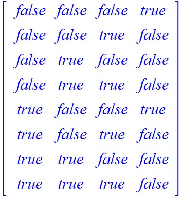
We can also use TruthTable to evaluate logical expressions for various values of inputs.

TruthTable(expression, l, options)

Figure 1.A.4: The TruthTable takes the pain out of constructing truth tables by hand.

Maple (Worksheet): Working with Truth Tables

> with(Logic):

> expression_1 := Random({a, b, c}, claues = 2)

expression_1 := ((a ∧ (¬b)) ∧ (¬c)) ∨ (((¬a) ∧ (¬b)) ∧ (¬c))

> TruthTable(expression_1)

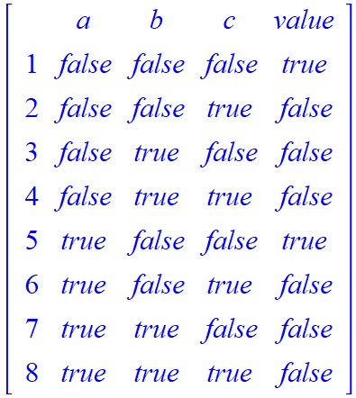
> TruthTable(expression_1, output = table)

> TruthTable(expression_1, output = Matrix)

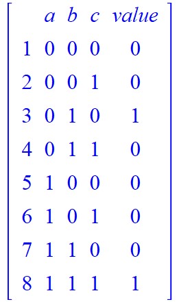
> TruthTable(expression_1, form = MOD2)

> expression_2 := Random({w, x, y, z}, clauses = 3):

> truth_table_1 := TruthTable(expression_2, form = MOD2, output = table):

> truth_table_1[1, 0, 0, 1]

> truth_table_2 := TruthTable(expression_2, output = table):

> truth_table_2[false, false, false, true]

true

Satisfiability

Sometimes, we may not be interested in analyzing a logical expression over every possible truth value assignment for its constituent parts. We may only want to know whether that expression is satisfiable, and we may only want one truth value assignment that yields a truth value of 1.

The Satisfiable, Satisfy, Tautology, and Contradiction functions are perfect for these purposes.

The Satisfiable function will determine if the given expression is satisfiable. If the expression is satisfiable, the Satisfy function will produce truth value assignments that yield a true value. When not satisfiable, the Satisfy function will return a value called NULL.

The Satisfiable function takes in an expression as a first argument to evaluate and various options that control how it determines satisfiability. These extra options are beyond the scope of this book.

The Satisfy function takes in an expression as a first argument, a set or list of names as an optional second argument, and the same various options accepted by the Satisfiable function. If the optional set or list of names is given to Satisfy, then Satisfy will return a satisfying set of values that includes every name in the set or list. This list of names must include all symbols provided in the given expression. Since it must include all names used in the expression anyway, we will not use this optional argument in this book.

For the next example, we’ll ramp up the number of names used in the expression to demonstrate why we would want to use Maple in the first place. Trying to this kind of analysis on an expression with five or more names will take a long time.

Satisfiable(expression)

Satisfy(expression)

Figure 1.A.5: These functions will help determine if an expression is satisfiable without having to do all the work associated with constructing a truth table.

Maple (Worksheet): Checking for Satisfiability

> with(Logic):

> expression := Random({a, b, c, d, e}, clauses = 6):

> Satisfiable(expression)

true

> Satisfy(expression)

{a = false, b = true, c = false, d = false, e = true}

> f_0 := a ∧ ¬a:

> Satisfiable(f_0)

false

> Satisfy(f_0)

Determining whether an expression is a tautology or a contradiction will go a long way in determining satisfiability.

The Tautology function takes in an expression as a first argument, and an optional second argument. This second argument must be an unevaluated name, meaning it must be a new variable that is being introduced into the Tautology function. If the expression is not a tautology, then p will contain a set of values that make the given expression false. Basically, the second argument will tell you why the given expression is not a tautology. If the expression is a tautology, then the second argument will receive the value NULL.

The Contradiction function works in nearly the same way. If the given expression is not a contradiction, then the second argument will contain a truth value assignment that makes the given expression evaluate to true.

Tautology(expression, p)

Contradiction(expression, p)

Figure 1.A.6: The Tautology and Contradiction functions can help determine satsifiability.

Maple (Worksheet): Testing for Tautologies and Contradictions

> with(Logic):

> expression := Random({a, b, c, d, e}, clauses = 3):

> T0 := p &implies (p &or q):

> F0 := q &and (r &and &not q):

> f_0 := a ∧ ¬a:

> Tautology(expression)

false

> Contradiction(expression)

false

> Tautology(expression, values_1):

> values_1

{a = false, b = false, c = true, d = true, e = false}

> Contradiction(expression, values_2)

{a = false, b = true, c = true, d = false, e = true}

> Tautology(T0, values_3):

> values_3

> Contradiction(F0, values_4):

> values_4

Testing for Logical Equivalence

Lastly, something we’ll want to test for often is logical equivalence. Once again, Maple offers functionality to easily test for equivalence.

The Equivalent function takes in two required arguments, both of which must be logical expressions. There is an optional third argument that acts a lot like the second argument for functions Tautology and Contradiction.That is to say, the optional third argument must be an unevaluated name. If the two expressions are not equivalent, then that third argument will be given an assignment of truth values that demonstrates why the two supplied arguments are not equivalent.

If the given two expressions are equivalent, then the optional third argument is given the value NULL.

Equivalent(exp_1, exp_2, values)

Figure 1.A.7: Captions for the above side content can offer more explanation about the topic being discussed.

Maple (Worksheet): Testing for Logical Equivalence

> with(Logic):

> exp_1 := p &implies q:

> exp_2 := (&not p) &or q:

> exp_3 := &not (p &or q):

> exp_4 := (&not p) &or (&not q)

> Equivalent(exp_1, exp_2)

true

> Equivalent(exp_3, exp_4)

false

> Equivalent(exp_1, exp_2, values_1):

> values_1

> Equivalent(exp_3, exp_4, values_2)

> values_2

{p = false, q = true}

This gives us a lot of tools that will make working with logical expressions much easier and less error-prone.

Simplifying Logical Expressions with Maple

Here, we’ll discuss the use of the BooleanSimplify function found within Maple’s Logic package. This function will take in a logical expression, and return an equivalent expression that is minimal.

BooleanSimplify(expression)

Figure 1.A.8: The BooleanSimplify function allows us to quickly simplify/minimize complicated logical expressions.

Maple (Worksheet): Simplifying Logical Expressions

> with(Logic):

> BooleanSimplify(¬(¬p or q))

p ∧ (¬q)

> BooleanSimplify(¬(¬((p ∨ q) ∧ r) ∨ ¬q))

q ∧ r

> BooleanSimplify((&not p &and &not q) &or (&not p &and q))

¬p

> BooleanSimplify(((p &or q) &and (p &or &not q)) &or q)

p ∨ q

Hiding Output With the : Operator

Before ending this section, we make note of one simple thing we can do to prevent Maple from outputting any additional information we don’t want to see.

We can place a colon : after each line if we want to execute that line of code, but don’t want Maple to show any output. This is particularly useful when importing packages. Some packages contain lots of definitions which can quickly clutter up our work space. In most of the above scripts, we’ve placed a colon : at the end of every line where we imported the Logic package. The only time we didn’t do this was in the first script where we actually wanted to see what was available in the package.

The Book ofFoundational Mathematics

Mathematical Logic With Maple

Introducing the Logic Package

Maple (Worksheet): Importing the Logic Package

Operators

Functions

Using the Operators

Maple (Worksheet): Using the Logical Operators

Maple (Worksheet): Logic with the Default Operators

Generating Logical Expressions

Maple (Worksheet): Generating Logical Expressions

Constructing Truth Tables

Maple (Worksheet): Working with Truth Tables

Satisfiability

Maple (Worksheet): Checking for Satisfiability

Maple (Worksheet): Testing for Tautologies and Contradictions

Testing for Logical Equivalence

Maple (Worksheet): Testing for Logical Equivalence

Simplifying Logical Expressions with Maple

Maple (Worksheet): Simplifying Logical Expressions

Hiding Output With the : Operator

The Book of
Foundational Mathematics