Boards with Rooks and Bishops

One easy way to extend what we’ve talked about thus far is to ask ourselves what happens when we allow both rooks and bishops on the same board. How many ways can we place rooks and bishops on a board so that no piece is attacked by any other piece? The cell decomposition strategy has been working for us so far, so lets see what happens when we try doing it with two pieces.

Cell Decomposition with Two Types of Chess Pieces

When we first talked about cell decomposition, we were only dealing with rooks, so we had two cases to consider: what happens when a cell is restricted, and what happens when a cell has a rook?

With both rooks and bishops, we’ll have three cases to consider: what happens when a cell is restricted, when it has a rook, and when it has a bishop?

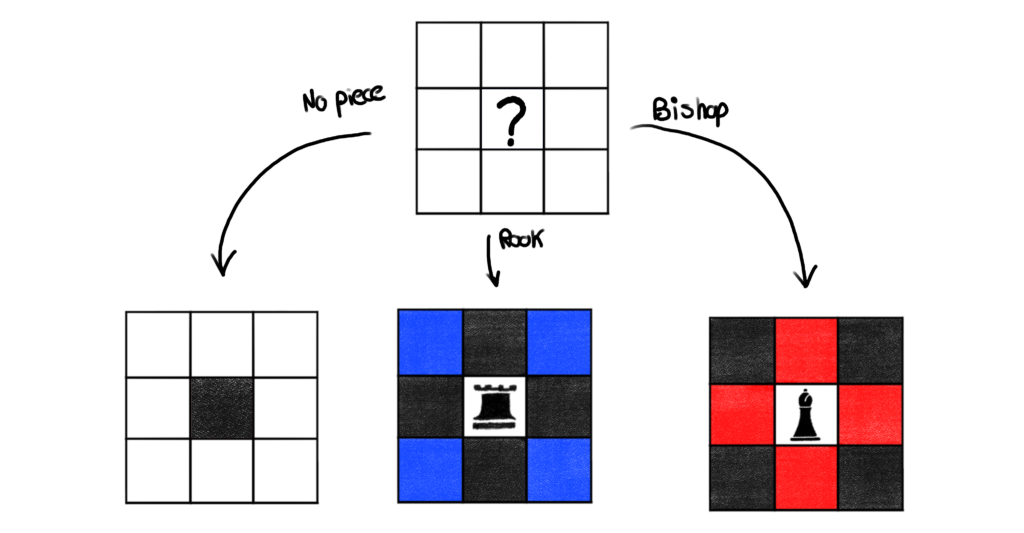
Let’s use a full 3-by-3 board to see what’s happening.

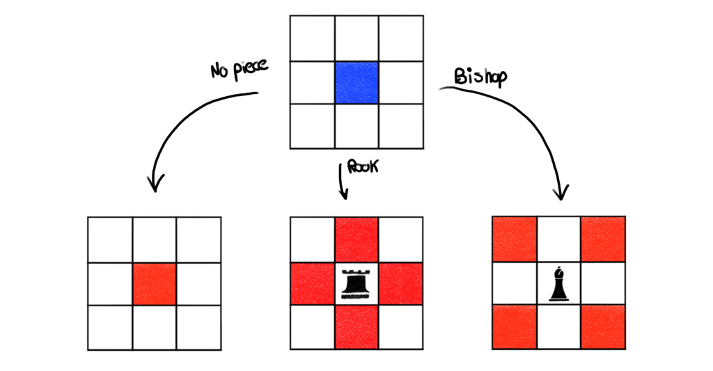
Just as we have been doing, red squares will be restricted from other pieces. Like usual, the row and column containing a rook are restricted from all other pieces, and any diagonal containing a bishop is restricted from all other pieces. This will prevent any piece from being captured by those pieces.

However, we run into a problem with this procedure. Let’s consider the middle board above with a rook placed in the center cell. While we can’t place any piece in any of the red cells, we can place any piece (including bishops) in the white corner cells. Placing a bishop in the upper left corner results in the following scenario.

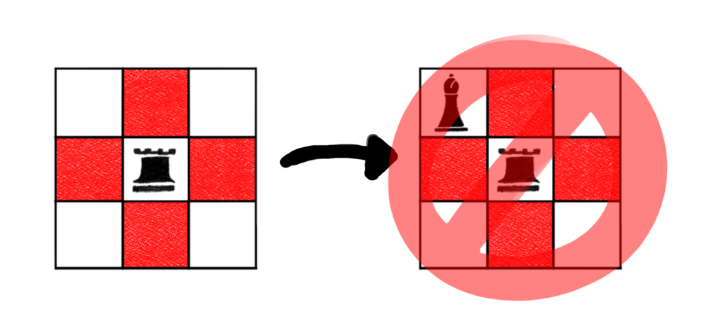
Doing this means that the rook is attacked by the bishop. This is precisely the situation we want to avoid in our counts. What happened? By restricting the middle row and middle column from any pieces, all we do is prevent any piece from being captured by the rook. This does not take into account any future placements of any pieces. While we prevent any piece from being captured by that rook, we did not prevent that rook from eventually being captured by a bishop.

Fixing the Procedure

In the situation depicted above, we want to to restrict any bishops from being placed in any of the corner cells, while still allowing rooks to be placed in the corner cells. This will prevent any piece from being captured while still allowing us to place any piece on the board in the future.

One way we could do this is to come up with a better color code. This is best done at the start so we can be consistent. For the rest of this article, we’ll use the following color coding scheme.

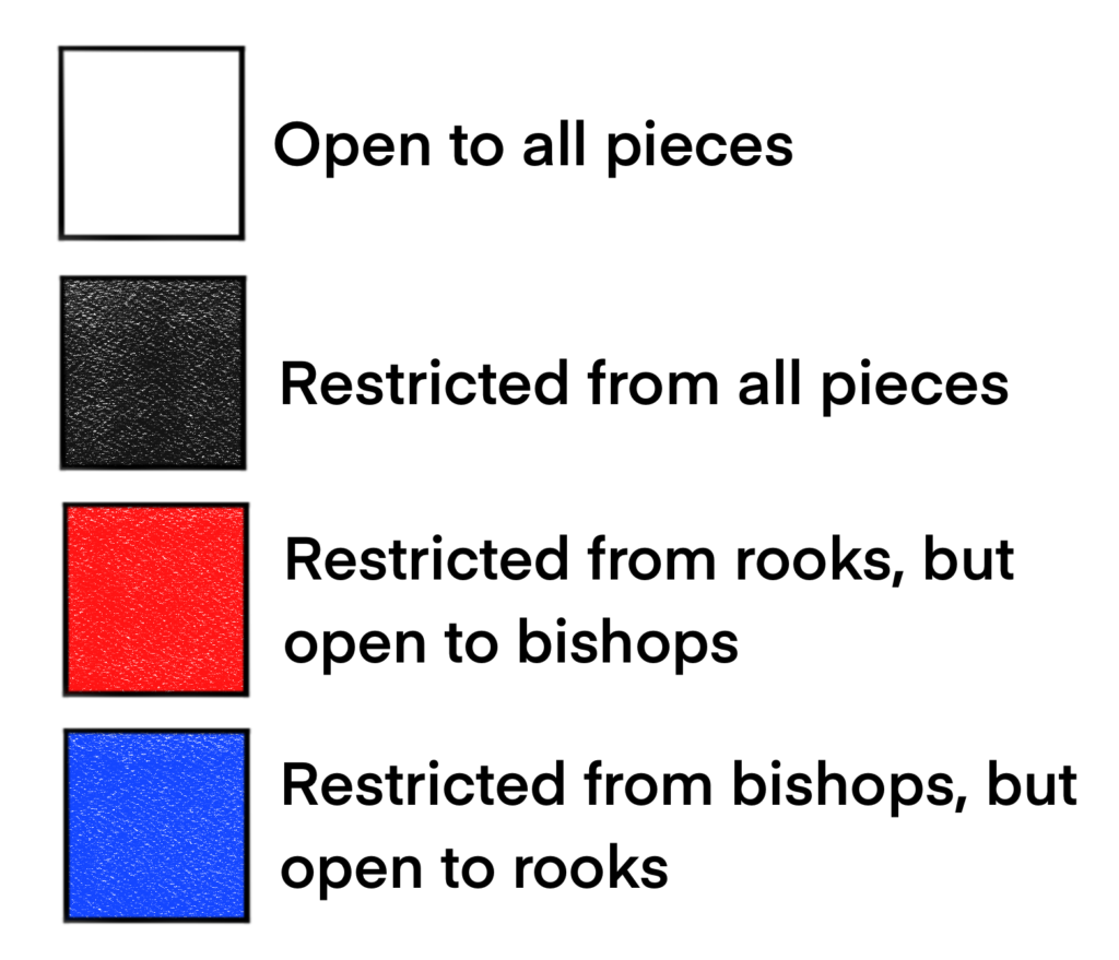
What this allows us to do is get a visual representation of what pieces are allowed on what squares. White cells are open to any piece. Black cells are restricted from all pieces. The red cells are restricted from rooks, but we will allow bishops to be placed on red cells. Similarly, rooks are allowed to be placed on blue cells, but bishops are not.

Using this scheme, we can now properly restrict cells as in the following picture.

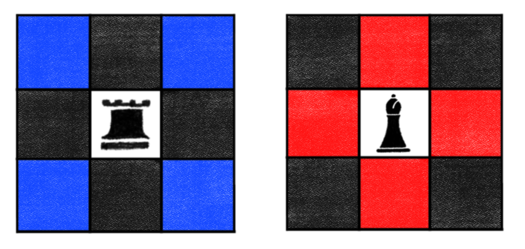
When we place a rook, we need to color all cells in the same row or column black to prevent any piece from being placed in those cells, and thus being attacked by the rook. We want to allow rooks to be placed in the blue cells because that won’t lead to a capture, we only want to prevent bishops from being placed in those cells because those bishops will capture the rook we just placed.

Similarly, when we place a bishop, we color all cells of the diagonals containing the bishop black to prevent any piece from being attacked by the bishop. The cells in the same row and column can still have a bishop placement because that won’t lead to a capture. However, any rook placed in the red cells will capture the bishop, so we’ll restrict rooks from being placed in the red cells.

With this, we have the following cell decomposition.

Much better!

Chess Polynomials

How do we represent the generating function we’re trying to compute? For starters, it no longer makes sense to refer to these polynomials as just Rook Polynomials or just as Bishop Polynomials. Going forward, we can just refer to these kinds of polynomials as Chess Polynomials.

That still leaves the question of what these polynomials are going to look like. Let’s consider a very simple example.

Example: The Single 1-by-1 Cell

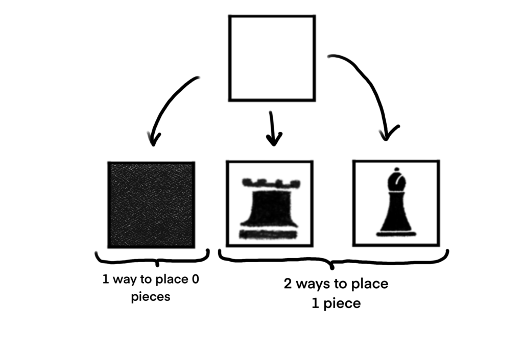
As usual, we see that there is exactly 1 way to place no pieces on the cell. We do see that there are 2 ways to place a single piece on this board. So using our previous methods we would say that the Chess Polynomial for this board is C(B, x) = 1 + 2x.

Here in this notation, we’re using B to represent the board and not the Bishop Polynomial, we’re using x as the variable, and we’re denoting the Chess Polynomial as C and not the board being used. This will make things a little more clear going forward, so this notation will be adopted.

Example: The 1-by-2 Board

That was simple enough, so let’s try something slightly more complicated, like the 1-by-2 board, which we’ll refer to as B_{1, 2}. Before showing what the decomposition would look like, let me tell you immediately that the Chess Polynomial for this board is C(B_{1, 2}, x) = 1 + 4x + x².

Using these types of polynomials, we should be able to immediately answer questions like how many ways are there to place 1 piece on the board. From looking at the coefficient of x in C(B_{1, 2}, x), we see that there are 4 ways. Similarly, because the coefficient of x² is 1, we see that there is 1 way to place two pieces on the board.

What if we asked how many ways are there to place 2 rooks? What if we asked how many ways there are to place 1 rook and 1 bishop (a total of 2 pieces?) What if we asked how many ways there are to place 2 bishops? Well, what exactly does that coefficient of 1 for x² mean? There are 3 possible combinations of 2 pieces, but only 1 valid way to place 2 pieces on the board at all. Which configuration is correct? It turns out that this representation is not too helpful in answering that particular question.

Here is the decomposition.

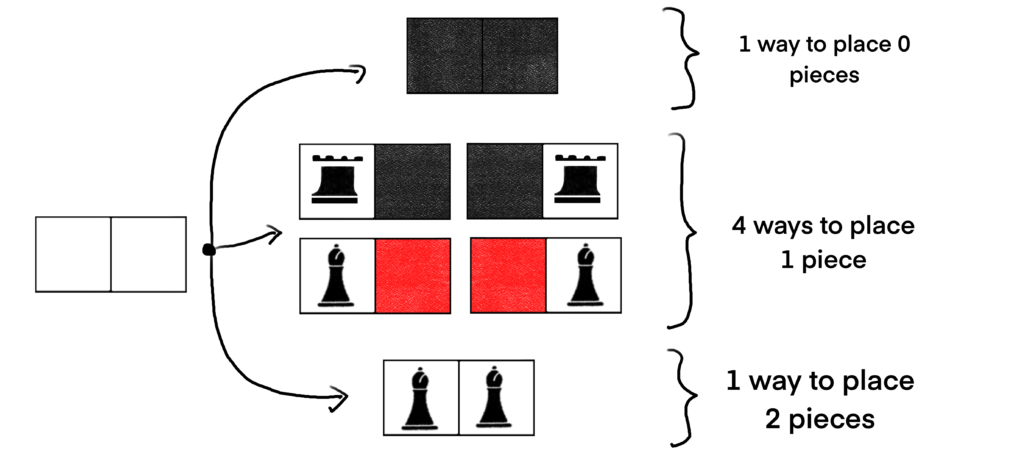
Based on this, we see that the 1 in front of x² actually refers to placing two bishops on the board. There are 0 ways to place two non-attacking rooks on this board, and there are 0 ways to place a non-attacking rook and bishop on this board.

Can we modify how we work with these polynomials to make this observation more apparent?

A Multivariate Generating Function

Let’s take one more look at the single cell board, but this time, let’s treat rooks and bishops separately.

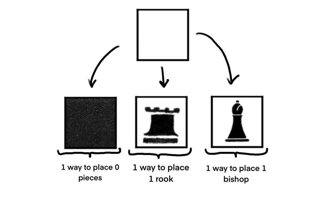
We want to keep our rook counts and bishop counts separate. We can do this by introducing another variable. The letter y is a good choice, so let’s use y to keep track of our bishop counts. We’ll still use x to keep track of our rook counts.

Using this scheme, we have that the Chess Polynomial for this board is now C(B, x, y) = 1 + x + y.

In this notation, we still use C to represent the Chess Polynomial, we still use B as the board, but now we include 2 letters in the notation, one for each distinct chess piece we’re using. This seems much better because now we know explicitly how many ways there are to place 1 rook separately from the number of ways of placing 1 bishop.

It’s worth noting that because we specify which letters we’re using in the polynomial, we could just as well write C(B, r, b) = 1 + r + b. Here, r is the variable keeping track of the rook placements, and b is naturally keeping track of the bishop placements. I like this a lot better than x and y, so going forward, I’ll use r and b.

Revisiting the 1-by-2 Board Example

Separating our counts based on what piece we’re using yields the following decomposition.

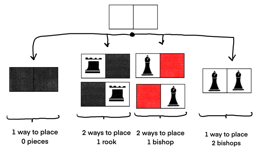
Now we can write C(B_{1, 2}, r, b) = 1 + 2r + 2b + 0r² + 0rb + 1b² = 1 + 2r + 2b + b².

Using this, it’s much easier to see what’s being counted by each of the coefficients.

Note that if we want to know how how many ways there are to place 1 piece on the board irrespective of what kind of piece it is, we can just add up the coefficients of the first powers. This gives us 2 + 2 = 4, which is what we got in our first attempt to write the Chess Polynomial for B_{1, 2}.

The Cell Decomposition Theorem Revisited

Just as we had to multiply the polynomial obtained from the board with a rook placement by x to account for the fact that there was an extra piece, we must do the same thing here. It’s not too hard to see that the new theorem will become the following:

Example: Chess Polynomial for the full 2-by-3 board

In this post, we realized just how tedious calculating the Bishop Polynomial for the full 3-by-3 board was, so in an effort to simplify our lives, we’ll just consider a full 2-by-3 board.

Decomposition 1

As always, we’ll start with the usual cell decomposition. Decomposing on the lower left corner gives us the following picture.

In this decomposition, we’ll still use B^* to denote the chessboard obtained by restricting the chosen cell from all pieces. B^R and B^B will of course denote the boards obtained by placed a rook and bishop respectively.

The Chess Polynomial for B^R should be easy enough to handle by inspection, so we’ll just note that we’re only considering the Chess Polynomial for the 1-by-2 subboard in the upper right corner. The Chess Polynomial for this subboard is C(B^R, r, b) = 1 + 2r + 1b + 0rb + 0r² + 0b² = 1 + 2r + b.

B^* and B^B still look a little too complicated to handle by inspection, so let’s decompose those boards as well.

Decomposition 2

Decomposing B^B on the upper-right corner cell yields the following situation.

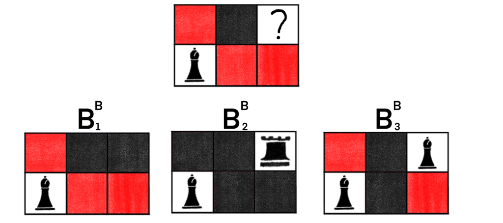
These boards are easy to handle by inspection.

C(B₁^B, r, b) = 1 + 0r + 3b + 2b² + 0b³ = 1 + 3b + 2b²
C(B₂^B, r, b) = 1 + 0r + 0b = 1
C(B₃^B, r, b) = 1 + 0r + 2b + 1b² = 1 + 2b + b²

Decomposition 3

Now we can decompose B^*, which we’ll do in the lower middle cell.

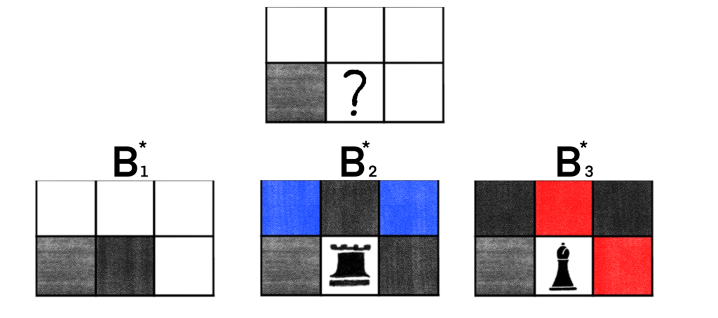
It looks like B₂^* and B₃^* are easily managed by inspection.
C(B₂^*, r, b) = 1 + 2r + 0b + 0r² = 1 + 2r
C(B₃^*, r, b) = 1 + 0r + 2b + 1b² = 1 + 2b + b²

Decomposition 4

We’ll probably want to decompose B₁^*, so let’s do that real quick.

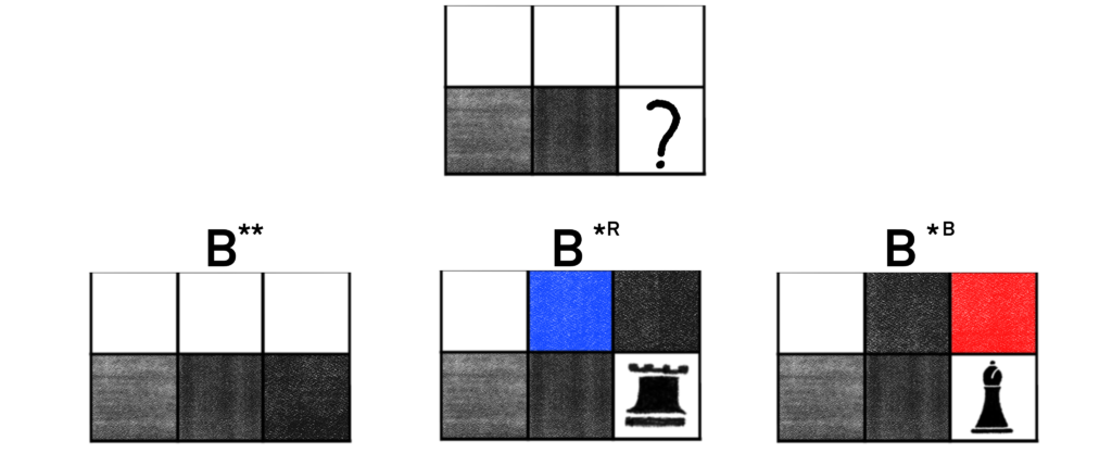
Ok, this will be our last decomposition. We have the following Chess Polynomials by inspection:
C(B^**, r, b) = 1 + 3r + 3b + 0r² + 3b² + 0rb + 1b³ = 1 + 3r + 3b + 3b² + b³
C(B^*R, r, b) = 1 + 2r + 1b + 0rb + 0r² = 1 + 2r + b
C(B^*B, r, b) = 1 + 1r + 2b + 0rb + 1b² = 1 + r + 2b

The Final Round of Calculations

Now we can calculate the Chess Polynomial for the full 2-by-3 board. Let’s recap. Here are the polynomials we still need to compute:

Here are the Chess Polynomials we figured out from inspection:

Working backwards, we can calculate the polynomial for B₁^*.

We can now calculate the polynomial for B^*.

We can calculate the polynomial for B^B.

And finally, we can calculate the polynomial for B.

Interpreting the Results

Using this generating function, we glean some information about the 2-by-3 board.
There are 6 ways to place a single rook on the board.
There are 6 ways to place a single bishop on the board.
There are 4 ways to place one non-taking rook and bishop on the board simultaneously.

If we ignore any terms with a factor of b, we are only left with r terms (and the constant), yielding the polynomial 1 + 6r + 6r², which is the Rook Polynomial for the 2-by-3 board.

Similarly, if we ignore the terms with a factor of r, we are only left with b terms (and the constant), yielding the polynomial 1 + 6b + 11b² + 6b³ + b⁴, which happens to be the Bishop Polynomial for the 2-by-3 board.

What’s Next?

At this point, we’ve got a lot of tools to help us calculate polynomials regarding one piece at a time, and now we can handle two pieces at a time with relative ease. We still need to automate this procedure, which requires some care, but is still going to be manageable. Stay tuned.