Introducing Bishop Polynomials

A “Quick” 3-by-3 Example

Just as we can count the number of ways to place some number of non-attacking rooks on a board, we can count the number of ways to place non-attacking bishops on a board. Bishops are perhaps the most closely related piece to rooks, so we expect the same general procedures to work with these pieces as well.

Our strategy will be the same as before: we decompose the board one cell at a time, considering cases where a bishop is placed at the cell, and when a bishop is not placed at the cell. As such, we will be using the Cell Decomposition Theorem as described in the second post of this series.

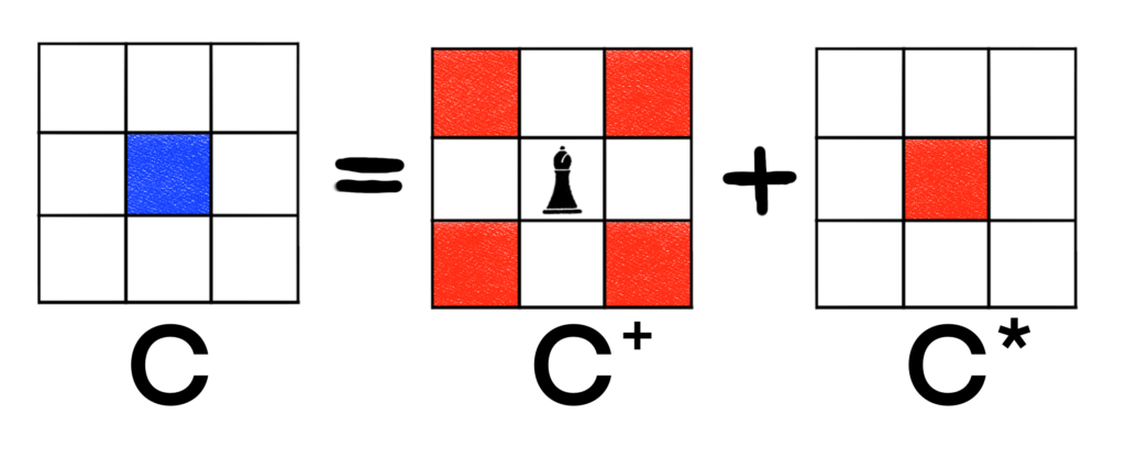
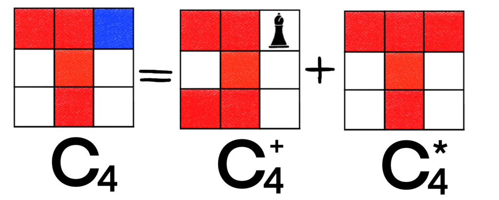
For the full 3-by-3 board, perhaps it makes sense to initially decompose on the center cell as shown below. Again, I’ll label the board with a bishop as C⁺ and I’ll label the board without a bishop as C^*. As before, whenever a cell is attacked by the bishop, I’ll shade it red. Any white cells remaining are free to have bishops placed on them.

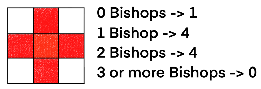
For C⁺, we’re left with a very simple board that we can handle by inspection.

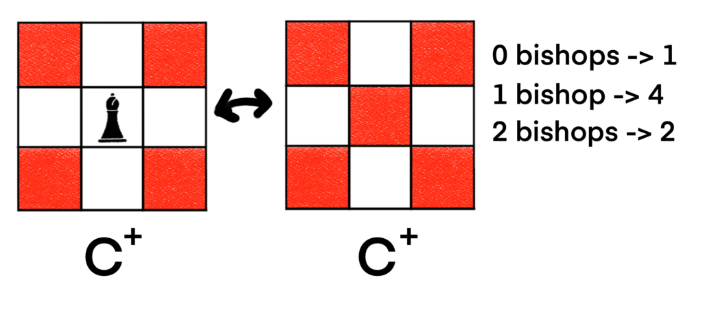
The Bishop Polynomial for C⁺ is B(C⁺, x) = 1 + 4x + 2x². Now that we have a handle on C⁺, we can work on C^*, which looks a little too complicated to handle by inspection. Let’s decompose that board and see what we get. Maybe it would be best if we decompose on a cell that is not a corner cell, as this will let us restrict more cells in the bishop placement board.

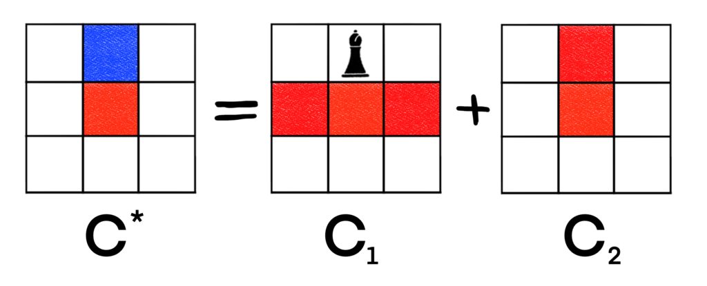
So, perhaps we could handle C₁ by inspection. It seems like we could place at most 3 non-attacking bishops on it, but that means we have to be careful to not overcount the number of ways to place 2 or 3 bishops. Maybe we should decompose it once more just to be safe. We’re definitely going to decompose C₂. This already looks like a pain, but we need to continue forward to get our answer.

We can decompose C₁ on the bottom middle piece to get the following.

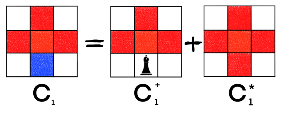
This is nice, because we’ve essentially produced the exact same board whether we place a bishop at the blue square or not. We can handle this board by inspection easily enough.

So we have that B(C₁⁺, x) = B(C₁^*, x) = 1 + 4x + 4x². Now we can start working on C₂. As said previously, we’ll decompose the board. Perhaps the lower middle cell would be best? Let’s see.

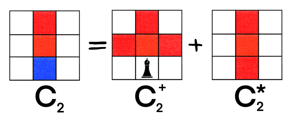
Notice that in this decomposition, we see that C₂⁺ will yield the exact same Bishop Polynomial as C₁⁺, so we have that B(C₂⁺, x) = B(C₁⁺, x) = 1 + 4x + 4x². Unfortunately, C₂^* still looks like a pain to do by inspection. We’ll need yet another decomposition. This board was very easy to handle with rooks, so why is it difficult with bishops? I’ll explain after we finish. Now, let’s just focus on the problem at hand. Hopefully, we’re almost done.

We can restrict two cells with a bishop by decomposing on a corner piece, so let’s do that.

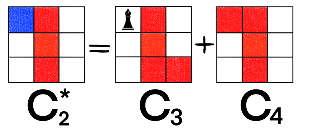
C₃ can be easily handled with inspection.

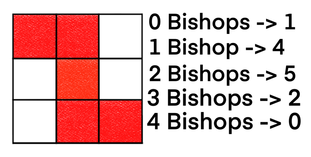
So, we have that B(C₃, x) = 1 + 4x + 5x² + 2x³. C₄ still looks too complicated to do by inspection, but if we decompose on the upper-right corner, we should be able to handle the next two boards by inspection. Let’s try.

We are now in a spot to handle both boards by inspection. For C₄⁺, we have the following.

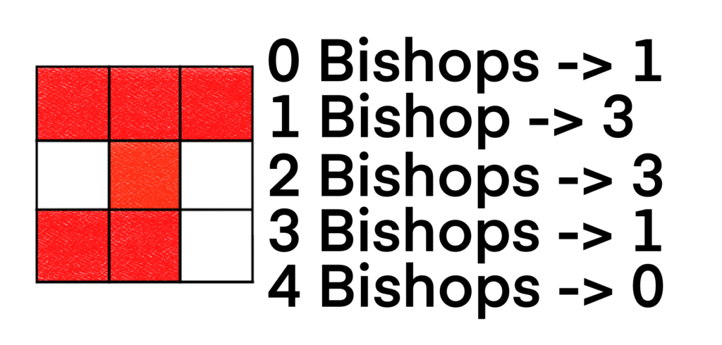
So B(C₄⁺, x) = 1 + 3x + 3x² + x³. For C₄^*, we have the following board.

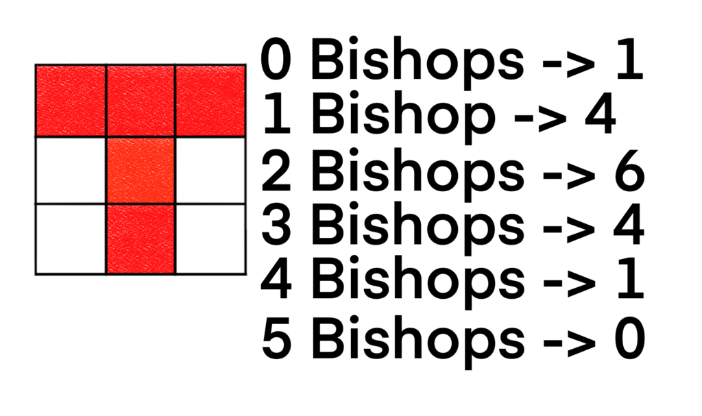
We get that B(C₄^*, x) = 1 + 4x + 6x² + 4x³ + x⁴.

We are finally in a position to calculate the Bishop Polynomial for our original board C. Before we proceed with the calculation, take a moment to appreciate the fact that we had to decompose the board many times to get to this point.

Let’s recap by showing all of the equations we got via the decomposition.

Here are the equations we figured out by inspection.

We can figure out C₄.

We can figure out C₂^*.

We can figure out C₂.

We can now figure out C₁.

We can also figure out C^*.

And for the grand finale, we can figure out C.

Relating Bishop Polynomials to Rook Polynomials

Let’s compare the Rook Polynomial for a full 3-by-3 board to the Bishop Polynomial we just calculated.

We can get a better understanding of what’s going on by examining bishop movement on a board.

Coordinates

We can label each row and column of a board to describe where a rook is placed. We can do the same thing for bishops, but since bishops move along diagonals, we may want to describe which diagonals on which a bishop is placed. This lets us more easily know if a bishop can be captured by another bishop.

For example, if two rooks share either a row coordinate or a column coordinate, they attack each other. When bishops share a diagonal, they attack each other, but how do we label the diagonals?

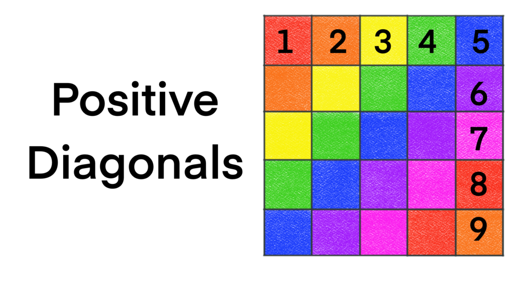
Just as there are two coordinates for rooks (rows and columns), there are two coordinates for bishops, which we’ll refer to as “positive diagonals” and “negative diagonals”. A positive diagonal is a diagonal formed by going right and up from a given square, as well as down and to the left. These diagonals are analogous to the graph of the line y = x in the xy-plane, which has a positive slope (hence the name positive diagonal.)

We can label positive diagonals by starting at the upper-left corner, and proceeding across the row. Once we hit the last column, we continue numbering the diagonals by going down the last column. Here is an example for the full 5-by-5 board. We’ll color all cells in the same positive diagonal the same color for clarity.

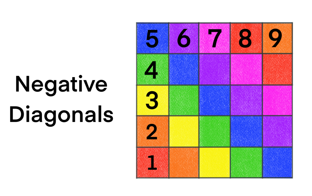
Similarly, a negative diagonal is formed by going up and to the left of a given cell, as well as down and to the right. These diagonals are analogous to the line y = -x graphed in the xy-plane which has a negative slope (hence the name negative diagonal.) To number negative diagonals, we start at the lower-left corner cell, and proceed up the column. Once we get to the top cell of the column we proceed to the right along the first row, stopping the numbering once we’ve reached the last column of the first row.

We illustrate the numbering scheme using the same full 5-by 5 board. Again, any cells belonging to the same negative diagonal will be colored the same.

Now that we have two different sets of coordinates for each cell, we can transform a board into a different board. Let’s start with the full 3-by-3 board we just finished working with in the previous section. For this board, there are 5 positive diagonals, and 5 negative diagonals, so we can make a 5-by-5 board where each row corresponds to a positive diagonal, and each column corresponds to a negative diagonal. We get the following result.

We color all squares in the 3-by-3 board green so we can see where they go under the transformation. In the upper-right corner of each cell in the 3-by-3 board is the positive diagonal to which the cell belongs. In the upper-left corner is the cell’s negative diagonal. In the 5-by-5 board, we want to restrict ay cells that were not present in the original board so they do not effect our analysis in any way. We’ll color those restricted cells red as we have been doing thus far.

It’s not hard to show that the Bishop Polynomial of the full 3-by-3 board is the same as the Rook Polynomial of the 5-by-5 transformation board, which goes a long way to explaining why we had so much work to do when calculating the Bishop Polynomial. We were essentially calculating the Rook Polynomial of a special 5-by-5 board.

Going forward, we’ll refer to any board that is formed by using this coordinate transform as a diagonalized board. This coordinate transform will be useful in future posts in this series about Rook Polynomials.

Red and Black Squares of a Chessboard

Typically, we don’t consider colors of the cells on a chessboard as they don’t affect the polynomial. With that said, while they don’t affect what the final polynomial is, considering colors can sometimes help us calculate the polynomial.

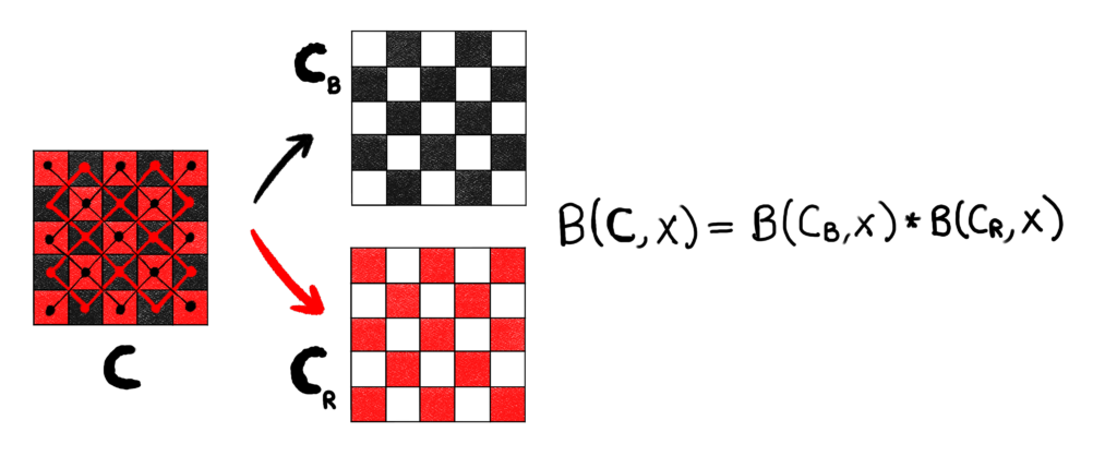
Take another moment to think about how bishops move on a chessboard. If we color all cells white, then nothing seems to be particularly interesting about how they move. However, once you color alternating cells red and black like a standard chessboard, something peculiar happens. A bishop on a red square will move along a diagonal, whose cells will all also be red. The next time it moves, it will be moving along some other diagonal, which again will have all red squares. This means that a bishop on a red square will always be on a red square. Thus, any bishop on a black square will never be attacked by a bishop on a red square. Similarly, any bishop on a red square will never be attacked by a bishop on a black square.

The implication here is that the red squares on a chessboard form a disjoint board from the black squares (with respect to bishop placements.) We can illustrate the situation to make it a little more clear.

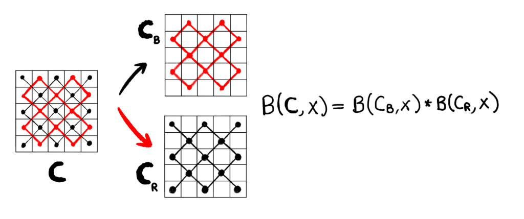
We could do the same thing for a board with all white squares as well. Once a bishop is placed on a cell, there are only some cells accessible to it on a board because bishops can only move to cells that share a diagonal with it. Off-diagonal cells are never attacked by a bishop. I just used a black and red board to make the observation obvious, but we can form these disjoint boards with any coloring of cells (except if a color depicts a restricted cell of course.)

It’s a standard result with Rook Polynomials that if two boards are disjoint, we can multiply the Rook Polynomial of both subboards to get the Rook Polynomial for the larger board. The same thing is true with bishops. To calculate the Bishop Polynomial of a large board, we can calculate the Bishop Polynomial of the “red board” and the “black board” separately, and then multiply the two polynomials together. That may have actually helped us work out the Bishop Polynomial for the full 3-by-3 board much faster, but cell decomposition is a more versatile method.

It’s worth stressing again that we can do this with a completely white board as well. We just need to determine which diagonals are inaccessible from a given bishop, no matter how many times it moves.

Automating the Calculation of Bishop Polynomials

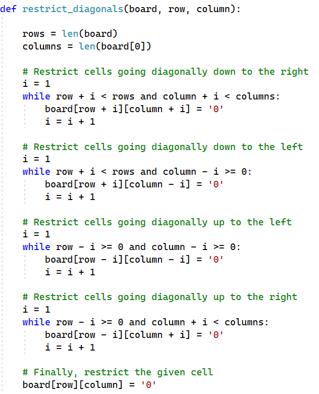
In a previous post, we went through a python script to calculate Rook Polynomials for us. We can also automate the calculation of Bishop Polynomials. We still use a recursive procedure that performs the cell decomposition needed to calculate the polynomial. The only difference is in how we restrict cells when we place a bishop. Other than that, the recursive procedure is the exact same.

Calculating Coordinates

We can essentially replace the cell restriction part of the rook_polynomial procedure with this function.

I’ve updated the script on my Github account, so you can view the entire thing here. At the time of this writing, I have two procedures: rook_polynomial and bishop_polynomial. In the future, I’ll be refactoring the code to make it easier to work with other chesspieces.

Transforming the Board

Since we have a procedure to calculate the Bishop Polynomial, we don’t need to diagonalize the given board, then calculate the diagonalized board’s Rook Polynomial. It does help to make sure you are getting consistent results, so we’ll add that functionality in as well.

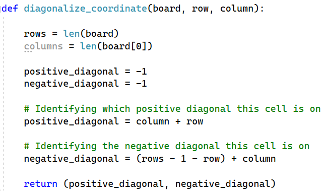
Here, we have a procedure that returns which positive diagonal and negative diagonal the given cell lies.

Here, we produce a diagonalized board from a given board.

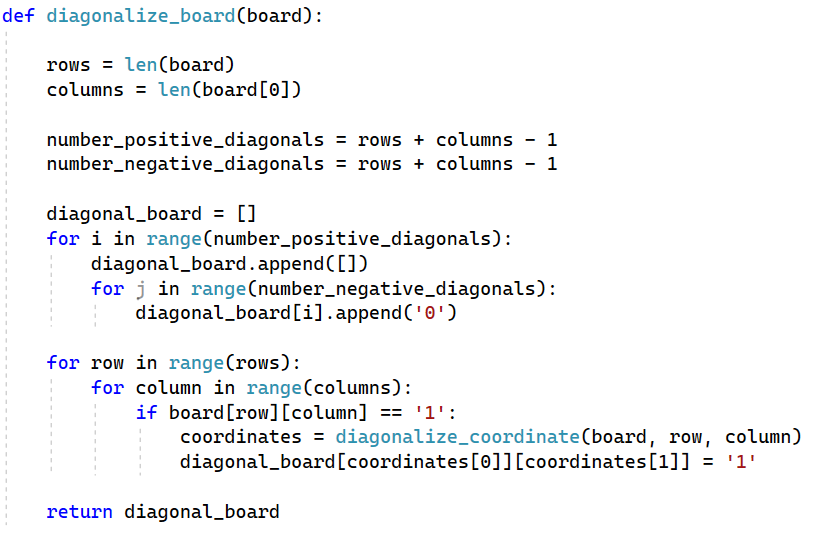
Since there are no comments in this block, I’ll briefly describe what’s going on. In the first iterated loop, we essentially populate a list of lists with the appropriate number of ‘0’ entries. It will produce a board with (rows + columns – 1) rows and columns since that is the number of positive diagonals and negative diagonals.

After we create the list of lists representing the diagonalized board, we then go though the original board looking for any ‘1’ entries. This will let us know which cells in the diagonalized board are unrestricted.

Once that’s done, we have a diagonalized board, so we return it.

Using the Script

Alright, now for the moment of truth. Does our script produce the correct polynomial. We already calculated the Bishop Polynomial for the full 3-by-3 board. Here are the results after running the program.

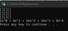
So for the full 3-by-3 board, our script produced the polynomial 1 + 9x + 26x² + 26x³ + 8x⁴. This is exactly what we got using cell decomposition, so the procedure seems to be working.

What’s Next?

I really want to refactor the code to make it easier to extend in the future. I also really want to make a version in Rust, so I’ll work on that as well, though this was not something I did for my thesis.

As far as my thesis is concerned the next steps will be looking at what happens when we have rooks and bishops on the same board. This means we’re going to taking a look at multivariate generating functions!

I won’t lie, I thought I was pretty clever for coming up with generating functions with two or more variables, and that I was doing something pretty unique. I recently started reading a book called “Analytic Combinatorics” by Philipe Flajolet and Robert Sedgewick which does cover the theory of multivariate generating functions, so that dashed my excitement a tiny bit, but it’s still a fascinating subject that I can’t wait to read more about!

Looking at rooks and bishops on the same board will naturally lead to us examining another chess piece. You may be able to guess what we’ll be looking at later, but I won’t spoil anything just in case. Stay tuned.