Physical Address
304 North Cardinal St.
Dorchester Center, MA 02124

I actually never took a graph theory course while I was in college, but seeing as it’s an extremely pervasive topic in discrete math (and math in general), I wanted to learn more. I worked through chapter 11 of Ralph Grimaldi’s book “Discrete and Combinatorial Mathematics” to get acquainted with the subject. I was particularly fond of section 11.6, which was about graph colorings and chromatic polynomials.
As I was working out several of the theorems from that section, I had the strangest feeling that what I was doing was extremely similar to other types of problems I’ve worked through before, but couldn’t quite put my finger on what those problems were. As it happens, I was also reviewing some of my probability notes from college, and came across license plate problems. One flash of insight later, I had a way of modeling license plate problems using graph colorings, and after working out some example problems, my answers all agreed with each other. In this post, I will be presenting this connection I made, and how I went about automating the process with Maple.
License plate problems are those problems where, given some set of symbols (typically uppercase letters A through Z, as well as the digits 0 through 9), and some possible restrictions on which positions can have which types of symbols, you have to count how many license plates exist satisfying the restrictions.
Here is the example I’ll be solving in this post:
Suppose license plates need to have 6 symbols, all of which come from the set {A, B, C, D, E, F} with the restriction that positions 2, 3, and 5 can only have symbols from {A, B, C}, and that position 2 must use a different symbol than position 4. How many such license plates are possible?
First, let me give a somewhat brief overview of all the tools I’ll use to solve this problem.
Let G = (V, E) be an undirected graph with vertex set V, and edge set E.
A proper coloring of G occurs when we color the vertices of G so that if {a, b} ∈ E, then the vertices a and b are colored differently. Basically, a proper coloring is any vertex coloring where adjacent vertices have different colors.
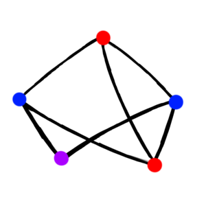
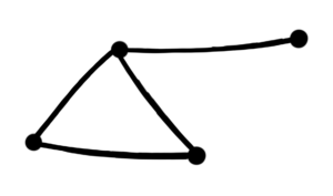
I like pictures, so here are two examples of graphs with properly colored vertices.
In the left-hand picture, there are 2 blue vertices, and only 1 vertex of the other colors. Notice that since the blue vertices are not connected by an edge, this is a proper coloring of this graph. In the right-hand picture, there are 2 red vertices, whereas there is only 1 vertex for the other 3 vertices. Again, since the red vertices are not connected by an edge, this is a proper coloring.
Properly coloring a complete graph requires as many colors as there are vertices, because every vertex is connected to every other vertex with an edge.
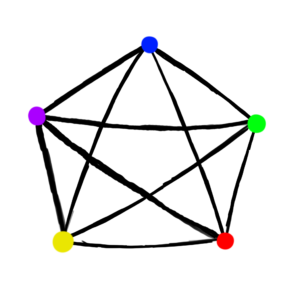
This property will be important later for solving our problem.
By definition, if 2 vertices are connected by an edge and they have the same color, then the vertices are not properly colored.
Notice that the 2 red vertices are connected by an edge, so this is an improperly colored edge.
In order to come up with a proper coloring of a graph, we can start by coming up with a proper coloring of a subgraph. Once we have a proper coloring of a subgraph, it’s usually a simple matter of making sure that any uncolored vertex gets a color that is not taken by any of its adjacent vertices.
For each proper coloring of a subgraph, there is a constant number of ways to properly color the remaining vertices.
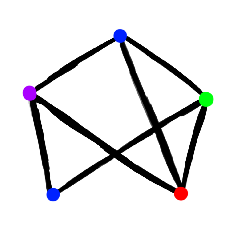
As an example, consider a graph with K3 as a subgraph. Here, we restrict each vertex to 1 of 4 colors, being red, green, blue, or purple. Our graph will have 4 vertices and 4 edges.
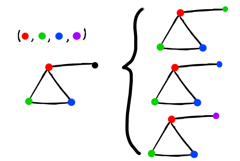
Notice that after we properly the color the subgraph K3, because we have 4 colors available, we can color the remaining vertex either green, blue, or purple. We can’t color it red because it’s adjacent to the red vertex.
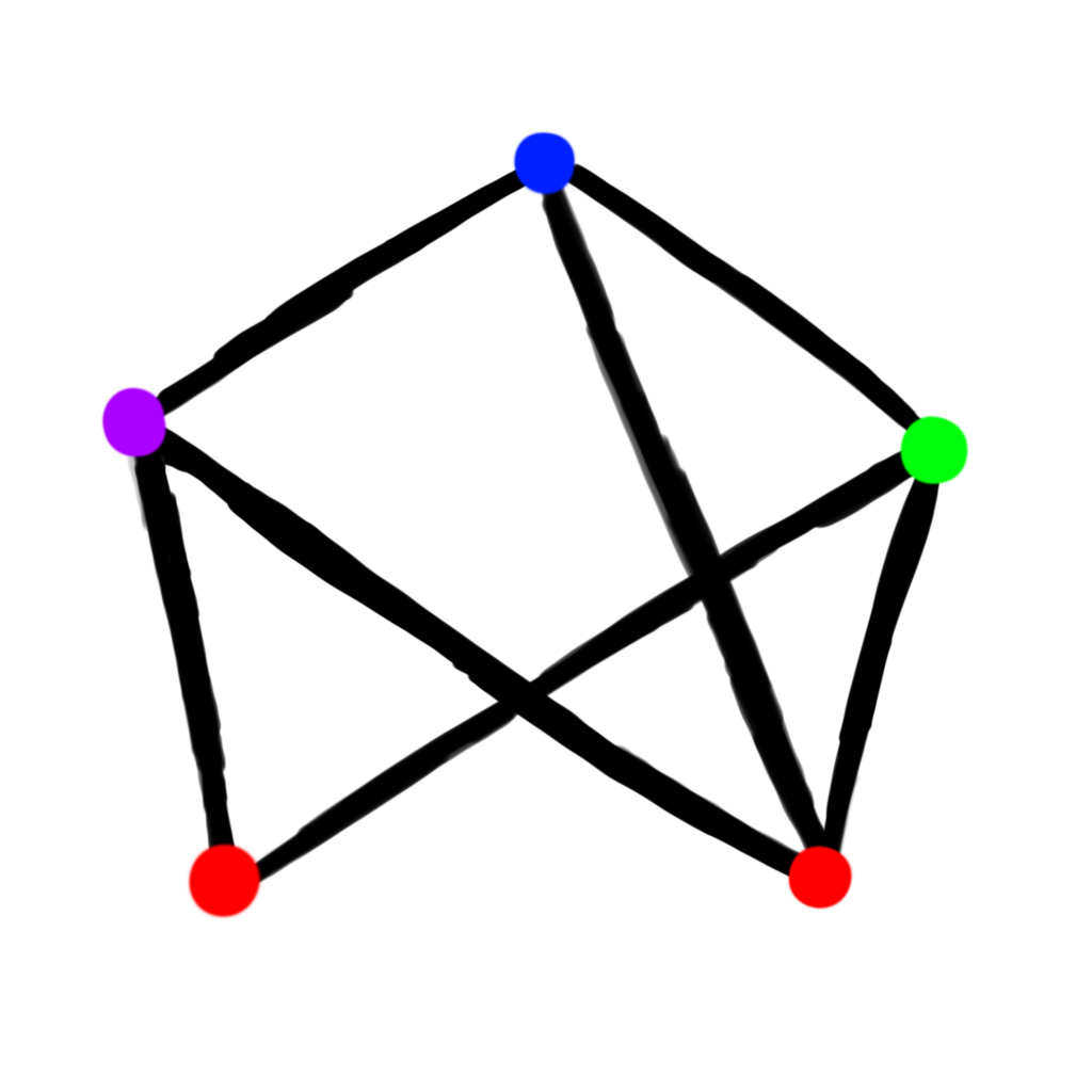
No matter how we properly color the subgraph of this graph, there will always be 3 ways to color the 4th vertex. If we add an additional edge to the 4th vertex, the number of options available decreases.
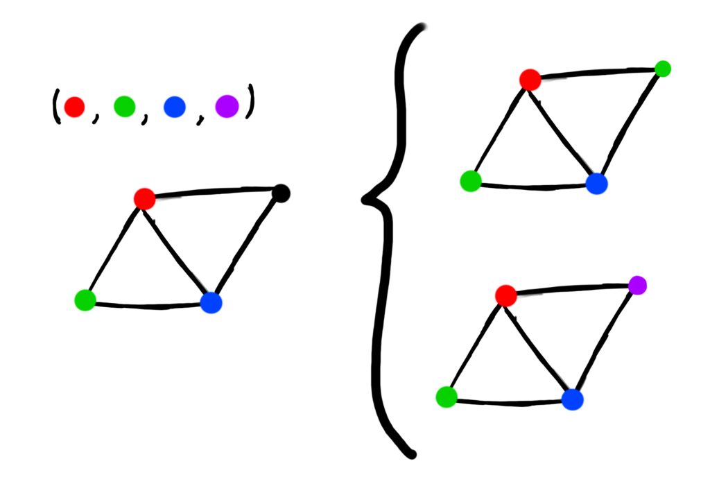
Here, because the 4th vertex is now adjacent to the red and blue vertices, we only have 2 valid colors left, those being green and purple.
Basically, the ratio of the number of proper colorings of the full graph to the number of proper colorings of the subgraph is just the number of ways to properly color the remaining vertices.
We can systematically determine the number of ways to properly color a graph by calculating its chromatic polynomial. Once we have the polynomial, we can simply evaluate the polynomial at any integer value representing the number of available colors.
Consider the 4-vertex graphs above. Here is the chromatic polynomial for such a graph.

λ(λ-1)2(λ-2)
The variable for the polynomial is λ. If we evaluate this polynomial at λ = 3, then we see that there are
(3)(3 – 1)2(3 – 2) = 3(4)(1) = 12 ways to properly color the graph using only 3 colors.
If we allow 4 colors (λ = 4), then there are (4)(4 – 1)2(4 – 2) = (4)(9)(2) = 72 ways to properly color the graph.
If we only allow 2 colors (λ = 2), then there are (2)(2 – 1)2(2 – 2) = 2(1)(0) = 0 ways to properly color the graph. Seeing as the maximum vertex degree is 3, this was expected.
Adding an additional edge has an effect on the chromatic polynomial as expected.
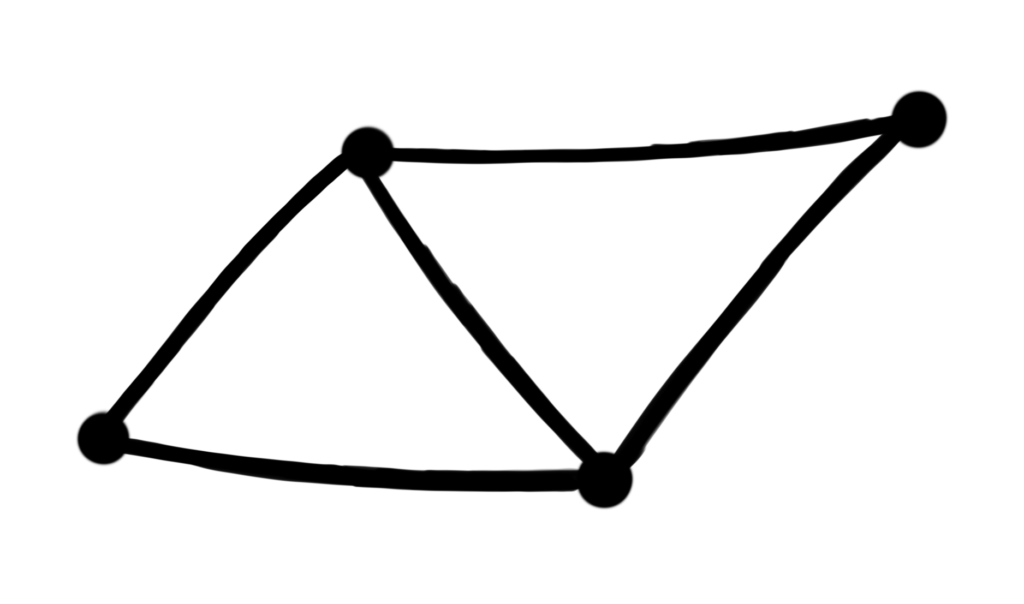
λ(λ-1)(λ-2)2
If we only allow 4 colors (λ = 4), then there are (4)(4 – 1)(4 – 2)2 = (4)(3)(4) = 48 ways to properly color this graph, much less than the 72 ways available for the previous graph with 4 colors.
As discussed earlier, the ratio of the number of proper colorings of the full graph to the number of proper colorings of the subgraph is just the number of ways to properly color the remaining vertices. If we can calculate the chromatic polynomial of the subgraph, then we can divide the polynomials to get the the chromatic polynomial of the remaining vertices.
Consider this graph again.
This graph has K3 as a subgraph, the chromatic polynomial of which is λ(λ – 1)(λ – 2).The chromatic polynomial of the whole graph is λ(λ-1)2(λ-2).
So, once we properly color the vertices of the subgraph, there are λ-1 ways to properly color the 4th vertex. If we have a palette of 4 colors, then after properly coloring the vertices of the K3 subgraph, there
4 – 1 = 3 ways to properly color the last vertex, which is what we saw above.
With this, we should be ready to finally model our license plate problem.
With all of this in mind, we’ll need to model each restriction on our license plates with cleverly constructed edges and vertices. Let’s restate the problem here for clarity: Suppose license plates need to have 6 symbols, all of which come from the set {A, B, C, D, E, F} with the restriction that positions 2, 3, and 5 can only have symbols from {A, B, C}, and that position 2 must use a different symbol than position 4. How many such license plates are possible?
Before we talk about the positions of the symbols on the license plate, let’s get a handle of the symbols themselves.
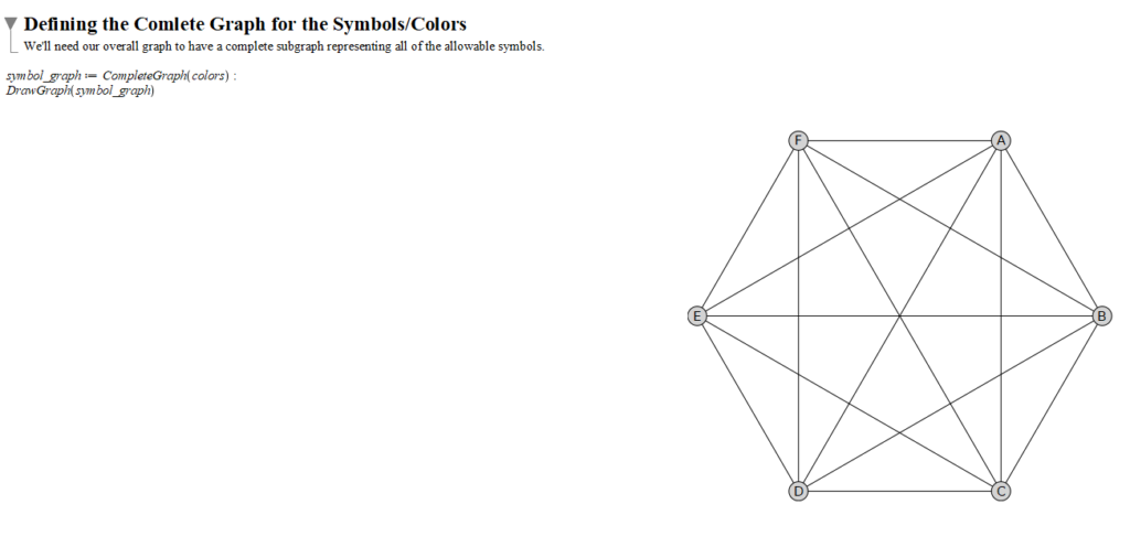
We can represent the symbols with a properly colored complete graph with as many vertices as there are symbols. By adding a properly colored complete graph, this allowed me to get as many colors needed while making sure it is still properly colored. This is because in a complete graph, every vertex is connected to every other vertex by an edge. The chromatic polynomial will take this into account.
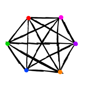
Here, we’ll let red represent A, green represent B, blue represent C, orange represent D, purple represent E, and pink represent F.
Our license plate has 6 positions that need to be assigned a letter. In terms of our chromatic polynomial, these vertices must be assigned a color. We’ll label these vertices for clarity.
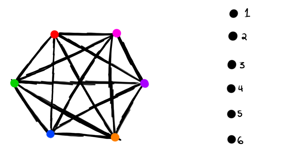
If we want to restrict a position from being assigned a symbol, that’s analogous to adding an edge between a restricted color vertex to an uncolored position vertex.
For example, Position 2 can only have an A, B, or C. This means that position 2 can’t have a D, E, or F. Based on our color coding from earlier, this means that the vertex labeled 2 can’t be colored orange, purple, or pink. To prevent this from happening in a proper coloring, we simply connect the orange, purple, and pink vertices to the vertex labeled 2 with an edge. The same restriction applies to position vertices 3 and 5.
In general, to prevent a symbol from being in a certain position, we connect that symbol’s color vertex to the appropriate position vertex with an edge.
This is what that graph looks like.
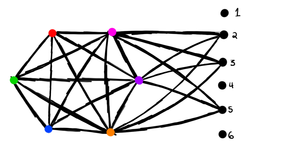
For our license plates, positions 2 and 4 must have different symbols. Analogously, this means that vertices labeled 2 and 4 can’t have the same color. Again, to prevent this from happening in a proper coloring, we add an edge between them.
In general, to prevent any two positions from having the same symbol, connect them with an edge.
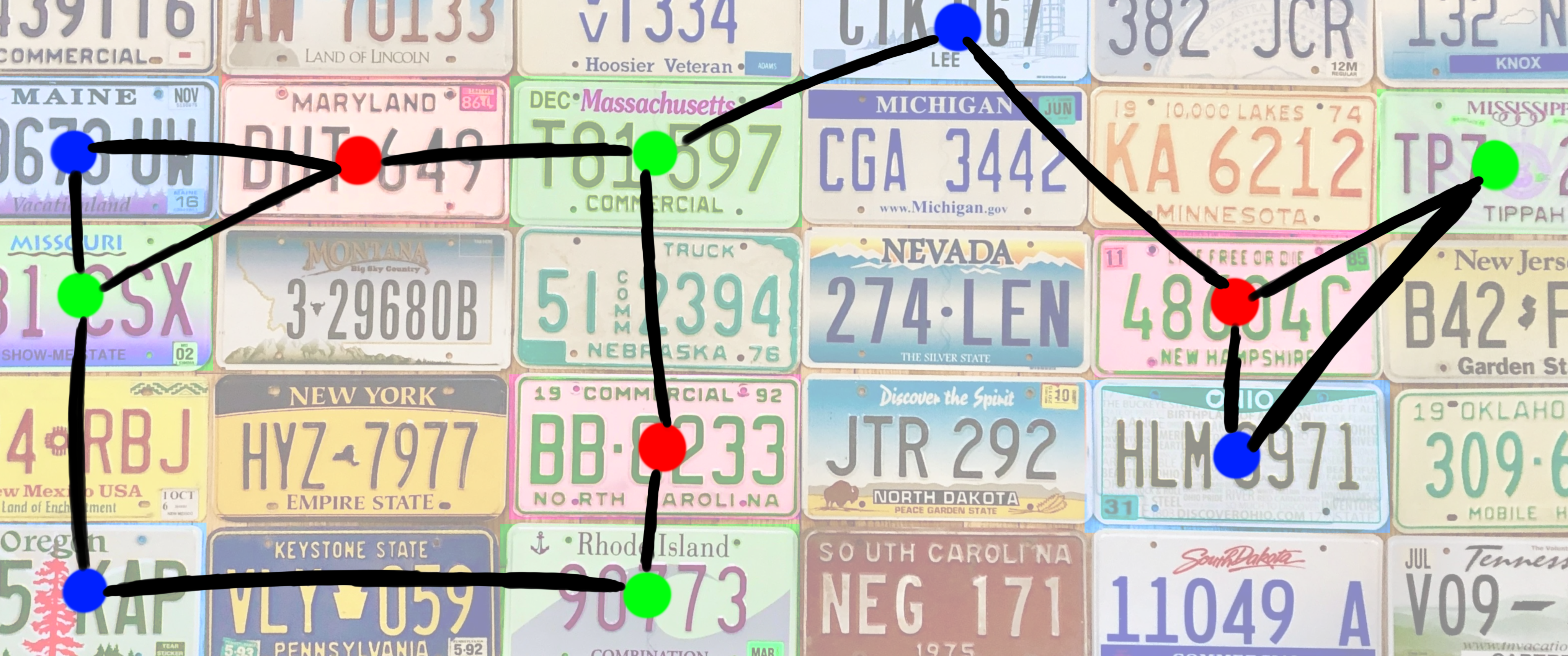
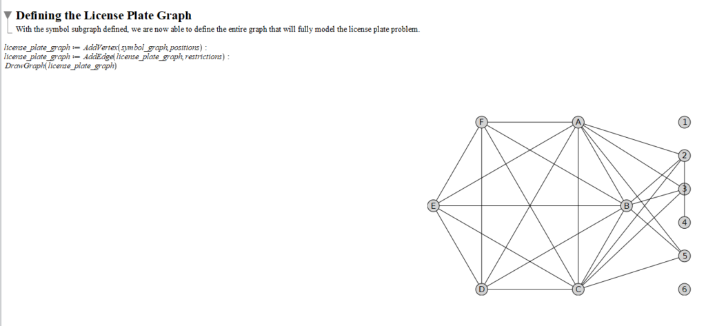
This is our final graph, representing the full license plate problem we’re trying to solve.
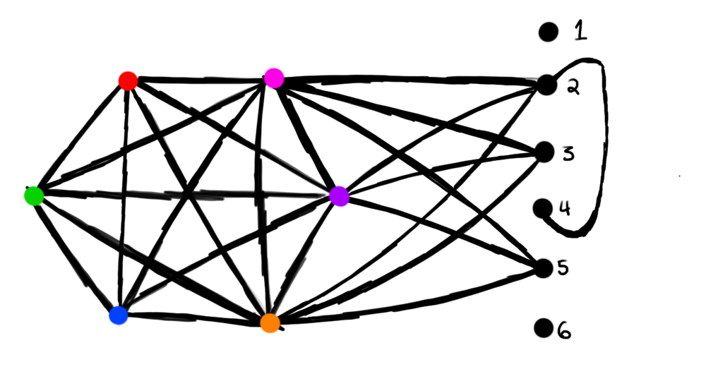
Though this is not a requirement for our particular problem, I figured I’d mention that in order to force any positions to have the same symbol, we can simply “coalesce” or “collapse” all of those vertices into one new vertex that represents all of them. We can then connect that new positional vertex to any number of colored vertices as needed.
Again, though not a restriction in our problem, I figured I would mention it for completeness. Here, we just connect every colored vertex to that positional vertex, except of course for the color representing the needed symbol.
Maple is an amazing tool, so instead of doing all of the tedious calculations by hand, I just let maple do it. I’ll detail the process here.
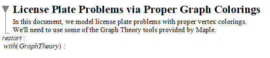
Naturally, I started the process by importing all necessary packages. Here, we just needed the GraphTheory package.
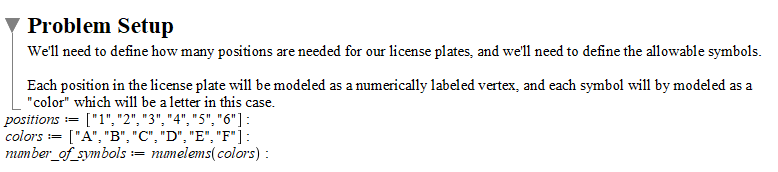
For our problem, we need to define a set of color vertices, and a set of position vertices. I decided to represent colors with uppercase letters, and positions on the license plate with integers. I also decided to capture the number of colors used, as that will be needed later.
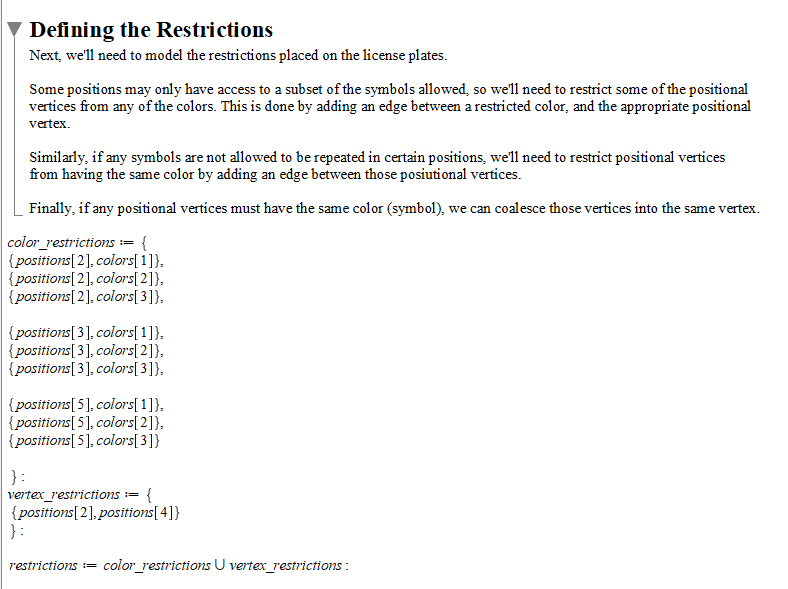
Next, I decided to add in the appropriate edges representing all of the restrictions needed for the problem. I just took the union of both sets afterwards in order to make adding them into the graph easier.
Using the CompleteGraph function makes adding the properly colored subgraph for the symbols easy. Capturing this graph in a variable will make computing its chromatic polynomial easy later. I drew each graph to the screen to double check that everything was working as expected.
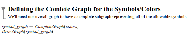
Without the graph, this is what the code looks like. The text in the previous image was hard to see for me, which is why I’m including it.
With the symbol subgraph made, in order to make the full graph representing our problem, we simply add the positional vertices, and any edges needed to get the needed restrictions in the graph. Throughout the development of this model, I’ve referred to the entire graph as a “license plate graph”, so I’ll adopt that terminology for the rest of this post.
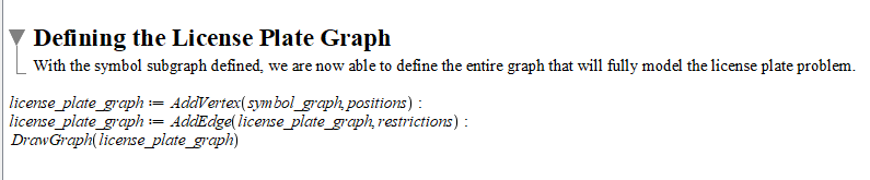
Again, the actual code is hard to see, so here is just the code without the image.
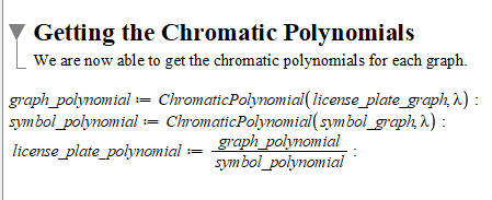
As discussed earlier, we want to count proper colorings of the positional vertices. So, we can divide the respective chromatic polynomials to get the desired result. Maple makes this extremely easy!
Because we only use 6 symbols, we need to evaluate the “license plate polynomial” calculated in the previous step at the number of symbols/colors used. We stored this value in a variable at the beginning of the document, so we just use Maple’s eval command to finish the problem.
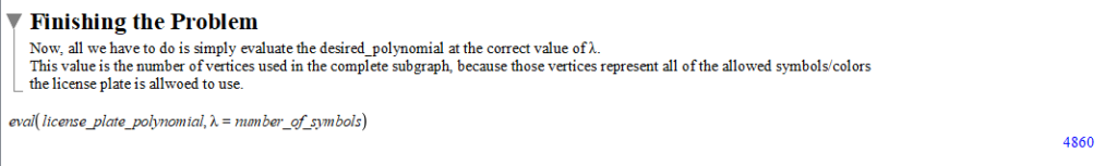
So, the answer is 4860. According to this model, there are 4860 license plates satisfying all of our desired restrictions.
Admittedly, this is a tad-bit overkill. Most people would probably calculate the answer this way:
6 * 3 * 3 * 5 * 3 * 6 = 4860.
There are no restrictions on the first position, so there are 6 choices of symbols that can be used in that position. Likewise for the sixth position. Positions 2, 3, and 5 only have access to 3 of the symbols, which is why we multiply by 3 three times. Position 4 can’t be the same as position 2, so there are only 5 possible choices for position 4.
Luckily, both answers are the same. It would be really awkward if, after all of that work, the answers were different.
The quick answer is that I could. As stated in the beginning of this post, I just finished learning about chromatic polynomials, and I saw a connection to license plate problems, so I wanted to flesh that connection out.
I had fun doing it, and I learned about a new Maple package I never used before. In college, I only used Maple for calculus and differential equations classes, so this application was a breath of fresh air.