Explaining and Solving the Three-Term Boundary Recurrence Problem

I took a discrete math class in college where I learned about generating functions and recurrence relations. I was amazed at how versatile these kinds of functions were in modeling combinatorial problems, so after I finished the class, I decided to learn more on my own. During my search for more reading material, I eventually discovered the book “Generatingfunctionology” by Herbert Wilf. As I was reading through the first chapter, I came across the three-term recurrence relation with boundary conditions, and struggled through the details of the method described in the book.

I was eventually able to get a grip on what was happening, but throughout the process, I doubted the validity of many of the steps taken through the solution as presented in the book. Luckily, after much careful thought, I was able to convince myself that every step taken was justified, but it was tricky. There were implicit assumptions made by the author, and there were some results being used that were not obvious to me as I was reading.

Furthermore, part of the general solution was left as an exercise for the reader, so this also left me scratching my head. I want to present my own solution to this exercise as well.

I love the book so far, and am looking forward to learning more, but I wanted to take an opportunity to clarify some of the parts of the solution that I initially had trouble with. Hopefully, this will help someone else struggling to get through that part of the book.

At the end of this post, I’ll provide two examples making use of the techniques presented in the book.

A Preliminary Result Regarding Quadratics

Let me take a moment to derive a basic result about quadratics before discussing the main problem.

Suppose we have the following quadratic equation, where none of the coefficients are 0.

\[ f(x) = a + bx + cx^2, a \neq 0, b \neq 0, c \neq 0 \]

Can the roots of this quadratic equation be 0? Let r₁ and r₂ be the roots of this quadratic equation. I’ll state the following theorem.

\begin{align} &\underline{\large{Theorem:}}\\ &\text{Consider the quadratic } cx^2 + bx + a \text{ where }a \neq 0, b \neq 0, c \neq 0\\ &\text{with roots } r_1 \text{ and } r_2\\ \\ &\text{Then } r_1 \neq 0 \text{, and } r_2 \neq 0 \end{align} \begin{align} &\underline{\large{Proof:}}\\ &\text{Since we know the roots are } r_1 \text{ and } r_2 \text{, we can factor the quadratic as such:}\\ \end{align} \begin{align} cx^2 + bx + a & = c(x – r_1)(x – r_2)\\ & = c[x^2 – (r_1 + r_2)x + r_1r_2]\\ & = cx^2 – c(r_1 + r_2)x + cr_1r_2\\ \end{align} \begin{align} &\text{This means that } a = cr_1r_2\\ &\text{Because } a \neq 0 \text{, } c \neq 0 \text{, this means that}\\ \end{align} \begin{align} & & cr_1r_2 &\neq 0\\ & \Rightarrow & r_1r_2 &\neq 0\\ & \Rightarrow & r_1 &\neq 0 \text{, } r_2 \neq 0\\ \end{align}

We actually didn’t even make use of the fact that b ≠ 0 in the proof, but it will be important later. We can get a more intuitive understanding of this fact by looking at some simple graphs.

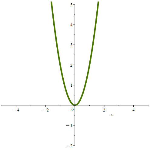
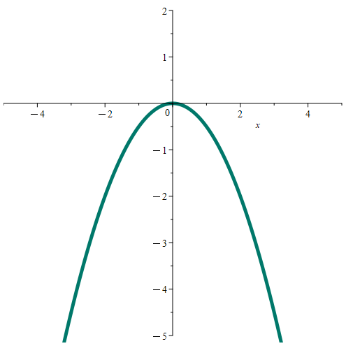
Here are some quadratics cx² + bx + a where c ≠ 0, but b = 0 and a = 0. These quadratics can of course be written simply as cx². Here, both roots are equal to 0.

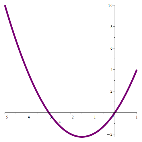
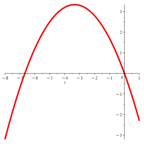
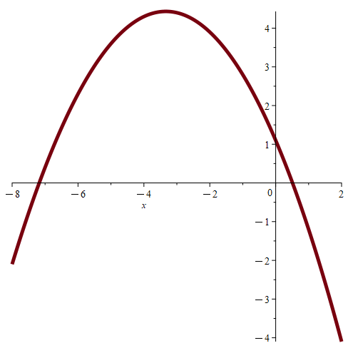
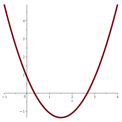
If we have quadratics cx² + bx + a where both c ≠ 0 and b ≠ 0, but with a = 0, then we can write this as cx² + bx + a = cx² + bx = x(cx + b) where only one root is 0, and the other root is non-zero. These quadratics look like the following parabolas. Note how only one point passes through the origin.

Now consider what quadratics of the form cx² + bx + a look like where c ≠ 0, b ≠ 0, and a ≠ 0. These are like the previous quadratics, except now we’re introducing a non-zero vertical shift to each parabola. This means that the parabola does not pass through the origin, and so neither root is equal to 0.

With this simple result taken care of, let’s start talking about the main problem.

The Three-Term Boundary Recurrence Problem

We want to find the general solution to the following problem as presented in the book.

\[ au_{n+1} + bu_n + cu_{n-1} = d_n\\ n \in \mathbb{N}\ where\ 0 < n < N\\ u_0 = u_N = 0 \]

Here, N is some constant natural number greater than 0. The coefficients a, b, and c are some given constants. Finally, the sequence

\[\{d_n\}_{n = 1}^{N-1}\]

is given in advance as well.

Before we tackle the problem, I want to make something clear. Here, we’re assuming the constants a, b, and c are all non-zero. If any one were 0, then we would effectively have a two-term recurrence, which defeats the entire purpose of dealing with a three-term recurrence in the first place. This assumption is not made explicit in the text, but will need to be understood in order to justify a future step.

Our goal is to determine the sequence

\[ \{u_n\}_{n=0}^N \]

that satisfies the given constraints.

The Preliminary Solution

You can read the details in the book, but eventually we get to the equation

\[ (a + bx + cx^2)U(x) = x[D(x) + au_1 + cu_{N-1}x^N] \]

where U(x) is the generating function for sequence

\[ \{u_n\}_{n=0}^N \]

and D(x) is the generating function for sequence

\[\{d_n\}_{n = 1}^{N-1}\]

Basically, we need to be able to solve for both u₁ and u_N-1. This means we need to solve a system of two equations (because we have two unknowns.)

There are two cases to consider.

Case: The roots of a + bx + cx² are distinct

To form a system of two equations, note that a + bx + cx² has two roots, which we’re considering to be distinct here. Let’s call these roots r₁ and r₂. If we substitute r₁ into x, we generate one equations as follows.

\[ \begin{alignat}{2} &&(a + b(r_1) + c(r_1)^2)U(r_1) & = (r_1)[D(r_1) + au_1 + cu_{N-1}(r_1)^N]\\ &\Rightarrow\quad &(0)U(r_1) & = (r_1)[D(r_1) + au_1 + cu_{N-1}(r_1)^N]\\ &\Rightarrow &0 & = (r_1)[D(r_1) + au_1 + cu_{N-1}(r_1)^N] \end{alignat} \]

This is where that preliminary result about the roots of quadratics comes into play. Because we know that c ≠ 0, b ≠ 0, and a ≠ 0, we know that r₁ ≠ 0. This means we can divide both sides of the equation by r₁ to get our first equation.

\[ \begin{alignat}{2} &&0 &= (r_1)[D(r_1) + au_1 + cu_{N-1}(r_1)^N]\\ &\Rightarrow\quad &0 &= D(r_1) + au_1 + cu_{N-1}(r_1)^N\\ &\Rightarrow &au_1 + cu_{N-1}(r_1)^N &= -D(r_1)\\ \end{alignat} \]

We can get our second equation using the exact same logic with the second root r₂. This gives us the following system of equations.

\[ \begin{align} au_1 + cu_{N-1}(r_1)^N &= -D(r_1)\\ au_1 + cu_{N-1}(r_2)^N &= -D(r_2)\\ \end{align} \]

By the nature of our recurrence, once we have u₁ and u_N-1, we just have to solve the recurrence for each individual term of the unknown sequence (u_n). Because N is a constant, this will be a finite process. Thus, we’ll be able to figure out what the unknown sequence is.

Case: The roots of a + bx + cx² are equal

This was the problem left to the reader. For my solution, I used a technique that was touched upon earlier in the book, which was to take a derivative of the generating function. Using the original equation, and a derivative of the equation will yield a system of two equations in two unknowns. Here is what I did.

First, because the roots are equal, I decided to rewrite the quadratic in factored form to make working with it a little bit easier.

\[ \begin{align} & & cx^2 + bx + a &= c(x – r)^2\\ & & &= c(x^2 – 2rx + r^2)\\ & & &= cx^2 – 2crx + cr^2\\ & \Rightarrow & b &= -2cr\ \text{and}\ a = cr^2 \end{align} \]

First, since both roots are equal, I just used r to refer the the root. Plugging this value in for x yields the following equation.

\[ \begin{align} & & (a + b(r) + c(r)^2)U(r) &= (r)[D(r) + au_1 + cu_{N-1}(r)^N]\\ &\Rightarrow & c(r – r)^2U(r) &= (r)[D(r) + au_1 + cu_{N-1}(r)^N]\\ &\Rightarrow & c(0)^2U(r) &= (r)[D(r) + au_1 + cu_{N-1}(r)^N]\\ &\Rightarrow & 0 &= (r)[D(r) + au_1 + cu_{N-1}(r)^N]\\ &\Rightarrow & 0 &= D(r) + au_1 + cu_{N-1}(r)^N\\ &\Rightarrow & au_1 + cu_{N-1}(r)^N &= -D(r) \end{align} \]

Now, as I previously said, I took the derivative of both sides with respect to x in order to generate the second equation needed. I substitute r for x after taking the derivative. Here is the result.

\[ \begin{align} & & \frac{d}{dx}[(a + bx + cx^2)U(x)] &= \frac{d}{dx}[x(D(x) + au_1 + cu_{N-1}x^N)]\\ & \Rightarrow & \frac{d}{dx}[c(x – r)^2U(x)] &= \frac{d}{dx}[x(D(x) + au_1 + cu_{N-1}x^N)]\\ & \Rightarrow & 2c(x – r)U(x) + c(x – r)^2U'(x) &= (D(x) + au_1 + cu_{N-1}x^N) + x(D'(x) + Ncu_{N-1}x^{N-1})\\ & \Rightarrow & 2c(r – r)U(r) + c(r – r)^2U'(r) &= D(r) + au_1 + cu_{N-1}r^N + rD'(r) + Ncu_{N-1}r^N\\ & \Rightarrow & 2c(0)U(r) + c(0)^2U'(r) &= D(r) + rD'(r) + au_1 + (N+1)cu_{N-1}r^N\\ & \Rightarrow & 0 &= D(r) + rD'(r) + au_1 + (N+1)cu_{N-1}r^N\\ & \Rightarrow & au_1 + (N+1)cu_{N-1}r^N &= -D(r) – rD'(r)\\ \end{align} \]

We finally have the two equations needed to solve for u₁ and u_N-1.

\[ \begin{align} au_1 + cu_{N-1}r^N &= -D(r)\\ au_1 + (N+1)cu_{N-1}r^N &= -D(r) – rD'(r) \end{align} \]

Example: Distinct Roots

Now that we have a handle on both cases, let’s look at an example that’s easier to grasp than the example presented in the book.

\[ \begin{align} &2u_{n+1} – 3u_n + u_{n-1} = d_n\\ &u_0 = u_5 = 0\\ &d_1 = 1,\ d_2 = 3,\ d_3 = 3,\ d_4 = 1 \end{align} \]

Here, we see that a = 2, b = -3, and c = 1. The roots of the quadratic cx² + bx + a are 1 and 2. Using this, we can solve for u₁ and u₄ using the solution we found when the roots are distinct.

First, let’s clearly state what D(x) is, because we’ll need to be able to evaluate it.

\begin{align} D(x) & = d_1x + d_2x^2 + d_3x^3 + d_4x^4\\ & = x + 3x^2 + 3x^3 + x^4 \end{align}

Now, we solve for u₁ and u₄,

\begin{align} & & au_1 + cu_{N-1}r_1^N = -D(r_1)\\ & & au_1 + cu_{N-1}r_2^N = -D(r_2)\\ \\ & \Rightarrow & (2)u_1 + (1)u_4(1)^5 = -D(1)\\ & & (2)u_1 + (1)u_4(2)^5 = -D(2)\\ \\ & \Rightarrow & 2u_1 + u_4 = -(1(1) + 3(1)^2 + 3(1)^3 + 1(1)^4)\\ & & 2u_1 + 32u_4 = -(1(2) + 3(2)^2 + 3(2)^3 + 1(2)^4)\\ \\ & \Rightarrow & 2u_1 + u_4 = -(1 + 3 + 3 + 1)\\ & & 2u_1 + 32u_4 = -(2 + 12 + 24 + 16)\\ \\ & \Rightarrow & 2u_1 + u_4 = -8\\ & & 2u_1 + 32u_4 = -54\\ \\ & \Rightarrow & u_1 = \frac{-101}{31} \text{ and } u_4 = \frac{-46}{31} \end{align}

Now that we have u₁, we can solve for u₂

\begin{align} & & 2u_2 – 3u_1 + u_0 &= d_1\\ & \Rightarrow & u_2 &= \frac{d_1 + 3u_1 – u_0}{2}\\ & & &= \frac{(3) + 3(\frac{-101}{31}) – (0)}{2}\\ & & &= \frac{-136}{31} \end{align}

We can also solve u₃.

\begin{align} & & 2u_5 – 3u_4 + u_3 &= d_4\\ & \Rightarrow & u_3 &= d_4 + 3u_4 – 2u_5\\ & & &= (1) + 3(\frac{-46}{31}) – 2(0)\\ & & &= \frac{-107}{31} \end{align}

Now we know the entire sequence.

\begin{align} u_0 &= 0\\ u_1 &= \frac{-101}{31}\\ u_2 &= \frac{-136}{31}\\ u_3 &= \frac{-107}{31}\\ u_4 &= \frac{-46}{31}\\ u_5 &= 0 \end{align}

We can double check by ensuring that the terms d₂ and d₃ are acquired by our recurrence using these values of u₀, u₁, u₂, u₃, u₄, u₅.

\begin{align} 2u_4 – 3u_3 + u_2 &= 2(\frac{-46}{31}) – 3(\frac{-107}{31}) + (\frac{-136}{31})\\ &= 3\\ &= d_3\\ \\ 2u_3 – 3u_2 + u_1 &= 2(\frac{-107}{31}) – 3(\frac{-136}{31}) + (\frac{-101}{31})\\ &= 3\\ &= d_2\\ \end{align}

Everything checks out, and our sequence works as desired!

Example: Equal Roots

Let’s check that my solution for the case of repeated roots works by considering the following example.

\[ \begin{align} &u_{n+1} – 2u_n + u_{n-1} = d_n\\ &u_0 = u_5 = 0\\ &d_1 = 1,\ d_2 = 1,\ d_3 = 2,\ d_4 = 3 \end{align} \]

Here, a = 1, b = -2, and c = 1, so the associated quadratic we have is cx² + bx + a = x² – 2x + 1, so both roots are equal to 1, so we’ll let r = 1 throughout this example.

Just as before, let’s take a moment to identify the generating function D(x) as well as D'(x), which we need in this example because the roots are repeated.

\begin{align} D(x) &= d_1x + d_2x^2 + d_3x^3 + d_4x^4\\ &= x + x^2 + 2x^3 + 3x^4\\ \\ D'(x) &= d_1 + 2d_2x + 3d_3x^2 + 4d_4x^3\\ &= 1 + 2(1)x + 3(2)x^2 + 4(3)x^3\\ &= 1 + 2x + 6x^2 + 12x^3\\ \end{align}

Now we can simply use the solution we found in the example to solve for u₁ and u₄.

\begin{align} & & au_1 + cr^Nu_{N-1} = -D(r)\\ & & cr^2u_1 + (N+1)cr^Nu_{N-1} = -D(r) – rD'(r)\\ \\ & \Rightarrow & (1)u_1 + (1)(1)^5u_4 = -D(1)\\ & & (1)(1)^2u_1 + (6)(1)(1)^5u_{4} = -D(1) – (1)D'(1)\\ \\ & \Rightarrow & u_1 + u_4 = -((1) + (1)^2 +2(1)^3 + 3(1)^4)\\ & & u_1 + 6u_4 = -((1) + (1)^2 +2(1)^3 + 3(1)^4) – (1 + 2(1) + 6(1)^2 + 12(1)^3)\\ \\ & \Rightarrow & u_1 + u_4 = -7\\ & & u_1 + 6u_4 = -28\\ \\ & \Rightarrow & u_1 = \frac{-14}{5} \text{ and } u_4 = \frac{-21}{5} \end{align}

Just as in the previous example, we can now solve for u₂.

\begin{align} & & u_2 – 2u_1 + u_0 &= d_1\\ & \Rightarrow & u_2 &= d_1 + 2u_1 – u_0\\ & & &= (1) + 2(\frac{-14}{5}) – (0)\\ & & &= \frac{-23}{5} \end{align}

Again, we solve for u₃.

\begin{align} & & u_5 – 2u_4 + u_3 &= d_4\\ & \Rightarrow & u_3 &= d_4 + 2u_4 – u_5\\ & & &= (3) + 2(\frac{-21}{5}) – (0)\\ & & &= \frac{-27}{5} \end{align}

Now we know the desired sequence of numbers.

\begin{align} u_0 &= 0\\ u_1 &= \frac{-14}{5}\\ u_2 &= \frac{-23}{5}\\ u_3 &= \frac{-27}{5}\\ u_4 &= \frac{-21}{5}\\ u_5 &= 0 \end{align}

Again, we can check that the recurrence yields d₂ and d₃ when using this sequence of numbers.

\begin{align} u_4 – 2u_3 + u_2 &= (\frac{-21}{5}) – 2(\frac{-27}{5}) + (\frac{-23}{5})\\ &= 2\\ &= d_3\\ \\ u_3 – 2u_2 + u_1 &= (\frac{-27}{5}) – 2(\frac{-23}{5}) + (\frac{-14}{5})\\ &= 1\\ &= d_2\\ \end{align}

Again, we get the expected results.

Conclusion

At this point, we’ve discussed some of the implicit assumptions, and preliminary results needed to understand the solution presented by Herbert Wilf in his book Generatingfunctionology. We also discussed a solution to a problem he posed, and came up with two example problems making use of the solution.

As stated previously, I’m enjoying working through his book, and would recommend it to anyone wanting to learn more about generating functions. I just wanted to clarify some subtle points that made understanding the solution much easier, and I wanted to propose my own solution to the problem he left for his readers.